Estimation des paramètres d’un modèle SIRD étendu pour la France

Le modèle proposé dans l’exemple Estimation des paramètres d’un modèle SIRD pour la France ne fonctionne pas très bien. Les données collectées sont erronées pour le recensement des personnes infectées. Comme les malades n’étaient pas testées au début de l’épidémie, le nombre officiel de personnes contaminées est en-deça de la réalité. On ajoute un paramètre pour tenir compte dela avec le modèle CovidSIRDc. Le modèle suppose en outre que la contagion est la même tout au long de la période d’étude alors que les mesures de confinement, le port du masque impacte significativement le coefficient de propagation. L’épidémie peut sans doute être modélisée avec un modèle SIRD mais sur une courte période.

Récupération des données

from datetime import timedelta
import warnings
import numpy
import pandas
from pandas import to_datetime
import matplotlib.gridspec as gridspec
import matplotlib.pyplot as plt
from aftercovid.data import extract_hopkins_data, preprocess_hopkins_data
from aftercovid.models import CovidSIRDc, rolling_estimation


data = extract_hopkins_data()
diff, df = preprocess_hopkins_data(data)
df.tail()

	deaths	confirmed	recovered	infected	safe
3/5/23	161435.968571	3.859429e+07	3.835907e+07	73569.0	2.840592e+07
3/6/23	161452.705049	3.860151e+07	3.836405e+07	76051.0	2.839844e+07
3/7/23	161475.657933	3.860777e+07	3.836844e+07	78139.0	2.839195e+07
3/8/23	161501.479928	3.861292e+07	3.837193e+07	79983.0	2.838659e+07
3/9/23	161512.000000	3.861851e+07	3.837547e+07	82286.0	2.838074e+07

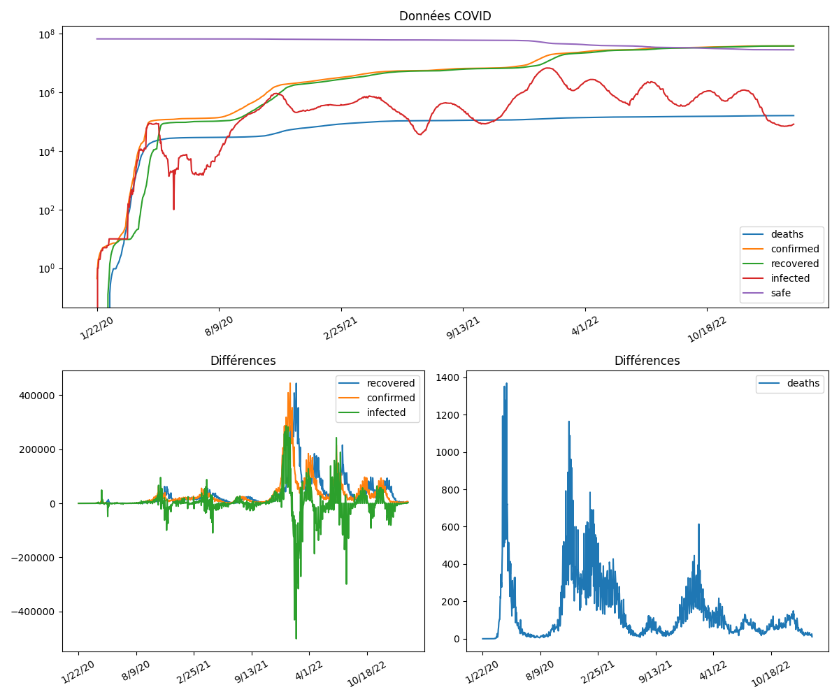
Graphes.

fig = plt.figure(tight_layout=True, figsize=(12, 10))
gs = gridspec.GridSpec(2, 2)
axs = []
ax = fig.add_subplot(gs[0, :])
df.plot(logy=True, title="Données COVID", ax=ax)
axs.append(ax)
ax = fig.add_subplot(gs[1, 0])
df[['recovered', 'confirmed', 'infected']].diff().plot(
    title="Différences", ax=ax)
axs.append(ax)
ax = fig.add_subplot(gs[1, 1])
df[['deaths']].diff().plot(title="Différences", ax=ax)
axs.append(ax)
for a in axs:
    for tick in a.get_xticklabels():
        tick.set_rotation(30)

Estimation d’un modèle

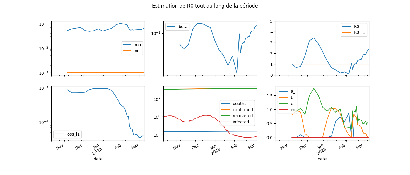
L’approche sur une fenêtre glissante suggère que le modèle n’est pas bon pour approcher les données sur toute une période, mais que sur une période courte, le vrai modèle peut être approché par un modèle plus simple. On note \(W^*(t)\) les paramètres optimaux au temps t, on étudie les courbes \(t \rightarrow W^*(t)\) pour voir comment évolue ces paramètres.

model = CovidSIRDc()
print(model.quantity_names)

data = df[['safe', 'infected', 'recovered',
           'deaths']].values.astype(numpy.float32)
print(data[:5])

X = data[:-1]
y = data[1:] - data[:-1]
dates = df.index[:-1]

Nlast = 150
X = X[-Nlast:]
y = y[-Nlast:]
dates = dates[-Nlast:]

['S', 'I', 'R', 'D']
[[6.7e+07 0.0e+00 0.0e+00 0.0e+00]
 [6.7e+07 1.0e+00 0.0e+00 0.0e+00]
 [6.7e+07 1.0e+00 0.0e+00 0.0e+00]
 [6.7e+07 2.0e+00 0.0e+00 0.0e+00]
 [6.7e+07 2.0e+00 0.0e+00 0.0e+00]]

Estimation.

# 3 semaines car les séries sont cycliques
dfcoef, model = rolling_estimation(
    X, y, delay=21, dates=dates, verbose=1, model_name='SIRDc')
dfcoef.head(n=10)

k=7 iter=500 loss=1704785237.333 l1=0.000852 coef=[5.51244745e-02 5.19949621e-02 1.00000000e-03 0.00000000e+00
 8.09872506e-01 1.00926077e+00] R0=1.0401832984503225 lr=1e-06 cn=1.2087649340185227e-07
k=14 iter=500 loss=1165412839.619 l1=0.000698 coef=[0.04327246 0.06082092 0.001      0.         0.96710839 0.92469848] R0=0.6999646643762756 lr=1e-06 cn=1.4434453617564753e-07
k=21 iter=500 loss=1178844208.762 l1=0.000698 coef=[ 5.39778013e-02  6.53644908e-02  1.00000000e-03 -9.52657144e-02
  9.07499570e-01  1.04273666e+00] R0=0.8133536580109411 lr=1e-06 cn=-1.4069096876251338e-05
k=28 iter=500 loss=1359292220.952 l1=0.000703 coef=[0.12636037 0.06908108 0.001      0.         0.1379203  0.81568362] R0=1.8030595968380614 lr=1e-06 cn=2.05851187091254e-08
k=35 iter=500 loss=1210804321.524 l1=0.000726 coef=[ 1.67114193e-01  5.15415035e-02  1.00088441e-03 -1.41187830e-07
  1.68445832e-05  1.50259685e+00] R0=3.1805595338150088 lr=1e-06 cn=-1.8537620774911145e-11
k=42 iter=500 loss=1611008585.143 l1=0.000867 coef=[1.67948691e-01 4.77998950e-02 1.00000000e-03 0.00000000e+00
 5.39498419e-08 1.75145072e+00] R0=3.441578943996731 lr=1e-06 cn=8.05221520493982e-15
k=49 iter=500 loss=1810886265.905 l1=0.000938 coef=[1.50366562e-01 5.08104331e-02 1.00000000e-03 0.00000000e+00
 2.78612093e-07 1.51619584e+00] R0=2.9022448343018 lr=1e-06 cn=4.158389442713024e-14
k=56 iter=500 loss=2028077641.143 l1=0.000931 coef=[1.34455267e-01 6.04573136e-02 1.00000000e-03 0.00000000e+00
 1.45366213e-04 1.08307078e+00] R0=2.1877830108133733 lr=1e-06 cn=2.1696449752151045e-11
k=63 iter=500 loss=1895819361.524 l1=0.000928 coef=[0.06683979 0.04910923 0.001      0.         0.6309379  0.93798974] R0=1.333881793864141 lr=1e-06 cn=9.416983536806788e-08
k=70 iter=500 loss=1862425843.810 l1=0.000939 coef=[ 4.02069759e-02  5.56717334e-02  1.00000000e-03 -4.45928894e-02
  1.04825453e+00  1.06866699e+00] R0=0.7094714316475454 lr=1e-06 cn=-6.492543582643944e-06
k=77 iter=500 loss=1496359399.619 l1=0.00083 coef=[ 3.00514092e-02  6.35628877e-02  1.00000000e-03 -5.82990282e-01
  1.01932781e+00  8.97664486e-01] R0=0.46545949661559693 lr=1e-06 cn=-8.677432296159342e-05
k=84 iter=500 loss=928947346.286 l1=0.000553 coef=[ 1.75432863e-02  8.83467338e-02  1.00008203e-03 -7.35717196e-01
  8.50612485e-01  1.01818909e+00] R0=0.19635043627184168 lr=1e-06 cn=-0.00010957177114874905
k=91 iter=500 loss=356274102.857 l1=0.000328 coef=[ 0.02919898  0.10103968  0.00100048 -0.56935693  0.36332277  0.37792229] R0=0.28615186874765003 lr=1e-06 cn=-8.483943987837672e-05
k=98 iter=500 loss=200768146.286 l1=0.000254 coef=[ 0.01199626  0.0940425   0.00100091 -0.86020174  0.08672528  0.35974727] R0=0.12621875893417625 lr=1e-06 cn=-0.00012824698718629722
k=102 iter=500 loss=87205924.571 l1=0.000148 coef=[ 9.67416281e-02  8.87796396e-02  1.00011945e-03 -1.19470285e-08
  1.53679117e-02  2.93083428e-01] R0=1.0775438587486592 lr=1e-06 cn=2.2919368101045423e-09
k=104 iter=500 loss=71490560.000 l1=0.000144 coef=[ 0.03444519  0.06742691  0.00100005 -0.67670331  0.61675021  0.95918409] R0=0.5033862442849031 lr=1e-06 cn=-0.00010080744146427216
k=106 iter=500 loss=14579483.429 l1=7.38e-05 coef=[ 5.29179598e-02  5.69480772e-02  1.00000000e-03 -2.20149647e-09
  8.33604622e-01  9.43033687e-01] R0=0.9131961301278865 lr=0.0001 cn=1.2441827207360772e-07
k=108 iter=16 loss=10862566.857 l1=6.23e-05 coef=[0.06011852 0.05286451 0.001      0.         0.75210348 0.90660207] R0=1.1161063325661933 lr=1e-06 cn=1.1225425011266694e-07
k=110 iter=20 loss=11031040.762 l1=6.31e-05 coef=[6.14755448e-02 5.56652277e-02 1.00000000e-03 0.00000000e+00
 7.11761267e-01 1.12668523e+00] R0=1.0848901042389643 lr=1e-06 cn=1.0623302493084362e-07
k=112 iter=500 loss=4659655.619 l1=4.39e-05 coef=[0.07431363 0.05412434 0.001      0.         0.4438066  0.53382489] R0=1.348109171997623 lr=0.0001 cn=6.623979042994271e-08
k=114 iter=13 loss=5098683.429 l1=4.49e-05 coef=[0.07741925 0.05454134 0.001      0.         0.45302667 0.67254934] R0=1.3939031747957633 lr=1e-06 cn=6.761592064674274e-08
k=116 iter=28 loss=5023411.429 l1=4.34e-05 coef=[0.08240906 0.05512022 0.001      0.         0.38079808 0.6240614 ] R0=1.4684378411188848 lr=1e-06 cn=5.683553430289065e-08
k=118 iter=423 loss=4922498.286 l1=4.29e-05 coef=[0.08365808 0.05553728 0.001      0.         0.3474347  0.62291308] R0=1.4796977738663863 lr=0.0001 cn=5.185592576587513e-08
k=120 iter=53 loss=3336917.714 l1=3.67e-05 coef=[0.10285107 0.0565727  0.001      0.         0.20173681 0.49140301] R0=1.7864553656131994 lr=1e-06 cn=3.010997156098567e-08
k=122 iter=7 loss=3278822.095 l1=3.59e-05 coef=[0.11171896 0.05711476 0.001      0.         0.14461697 0.49822973] R0=1.9223854012980193 lr=1e-06 cn=2.1584622533530204e-08
k=123 iter=500 loss=3303460.571 l1=3.6e-05 coef=[0.11124199 0.05730113 0.001      0.         0.15801755 0.521657  ] R0=1.9080590076706614 lr=0.0001 cn=2.3584709117652187e-08
k=124 iter=475 loss=3539710.476 l1=3.76e-05 coef=[0.1110337  0.05755336 0.001      0.         0.15477681 0.58551918] R0=1.8962822278431477 lr=0.0001 cn=2.3101016726841352e-08
k=125 iter=207 loss=3544424.000 l1=3.77e-05 coef=[0.11122954 0.05724697 0.001      0.         0.15228159 0.56742783] R0=1.9096193502222152 lr=0.0001 cn=2.272859563035071e-08
k=126 iter=4 loss=3542836.952 l1=3.89e-05 coef=[0.12769099 0.05983655 0.001      0.         0.08778711 0.47485418] R0=2.0989188727146773 lr=1e-06 cn=1.3102554100980128e-08
k=127 iter=247 loss=3861068.952 l1=4.06e-05 coef=[0.1361947  0.06070814 0.001      0.         0.04790946 0.51141619] R0=2.2070781900736423 lr=0.0001 cn=7.150665309228099e-09
k=128 iter=52 loss=3870073.524 l1=3.98e-05 coef=[0.14485405 0.06274423 0.001      0.         0.00852612 0.52687529] R0=2.2724262377044973 lr=1e-06 cn=1.2725554330299687e-09
k=129 iter=9 loss=3967654.857 l1=3.98e-05 coef=[1.48831720e-01 6.16830460e-02 1.00000000e-03 0.00000000e+00
 6.69211248e-05 5.51805375e-01] R0=2.374353659187325 lr=1e-06 cn=9.988227574941034e-12

	k	loss	loss_l1	it	R0	lr	correctness	beta	mu	nu	a	b	c
date
11/6/22	7	1.704785e+09	0.000852	500	1.040183	0.000001	1.208765e-07	0.055124	0.051995	0.001000	0.000000e+00	8.098725e-01	1.009261
11/13/22	14	1.165413e+09	0.000698	500	0.699965	0.000001	1.443445e-07	0.043272	0.060821	0.001000	0.000000e+00	9.671084e-01	0.924698
11/20/22	21	1.178844e+09	0.000698	500	0.813354	0.000001	-1.406910e-05	0.053978	0.065364	0.001000	-9.526571e-02	9.074996e-01	1.042737
11/27/22	28	1.359292e+09	0.000703	500	1.803060	0.000001	2.058512e-08	0.126360	0.069081	0.001000	0.000000e+00	1.379203e-01	0.815684
12/4/22	35	1.210804e+09	0.000726	500	3.180560	0.000001	-1.853762e-11	0.167114	0.051542	0.001001	-1.411878e-07	1.684458e-05	1.502597
12/11/22	42	1.611009e+09	0.000867	500	3.441579	0.000001	8.052215e-15	0.167949	0.047800	0.001000	0.000000e+00	5.394984e-08	1.751451
12/18/22	49	1.810886e+09	0.000938	500	2.902245	0.000001	4.158389e-14	0.150367	0.050810	0.001000	0.000000e+00	2.786121e-07	1.516196
12/25/22	56	2.028078e+09	0.000931	500	2.187783	0.000001	2.169645e-11	0.134455	0.060457	0.001000	0.000000e+00	1.453662e-04	1.083071
1/1/23	63	1.895819e+09	0.000928	500	1.333882	0.000001	9.416984e-08	0.066840	0.049109	0.001000	0.000000e+00	6.309379e-01	0.937990
1/8/23	70	1.862426e+09	0.000939	500	0.709471	0.000001	-6.492544e-06	0.040207	0.055672	0.001000	-4.459289e-02	1.048255e+00	1.068667

Saving the results.

df.index = to_datetime(df.index)
dfcoef.index = to_datetime(dfcoef.index)
df.to_csv("plot_covid_france_sird_cst.data.csv", index=True)
dfcoef.to_csv("plot_covid_france_sird_cst.model.csv", index=True)

somewhereaftercovid_39_std/aftercovid/examples/plot_covid_france_sird_cst.py:103: UserWarning: Could not infer format, so each element will be parsed individually, falling back to `dateutil`. To ensure parsing is consistent and as-expected, please specify a format.
  df.index = to_datetime(df.index)
somewhereaftercovid_39_std/aftercovid/examples/plot_covid_france_sird_cst.py:104: UserWarning: Could not infer format, so each element will be parsed individually, falling back to `dateutil`. To ensure parsing is consistent and as-expected, please specify a format.
  dfcoef.index = to_datetime(dfcoef.index)

Fin de la période.

dfcoef.tail(n=10)

	k	loss	loss_l1	it	R0	lr	correctness	beta	mu	nu	a	b	c
date
2023-02-25	118	4.922498e+06	0.000043	423	1.479698	0.000100	5.185593e-08	0.083658	0.055537	0.001	0.0	0.347435	0.622913
2023-02-27	120	3.336918e+06	0.000037	53	1.786455	0.000001	3.010997e-08	0.102851	0.056573	0.001	0.0	0.201737	0.491403
2023-03-01	122	3.278822e+06	0.000036	7	1.922385	0.000001	2.158462e-08	0.111719	0.057115	0.001	0.0	0.144617	0.498230
2023-03-02	123	3.303461e+06	0.000036	500	1.908059	0.000100	2.358471e-08	0.111242	0.057301	0.001	0.0	0.158018	0.521657
2023-03-03	124	3.539710e+06	0.000038	475	1.896282	0.000100	2.310102e-08	0.111034	0.057553	0.001	0.0	0.154777	0.585519
2023-03-04	125	3.544424e+06	0.000038	207	1.909619	0.000100	2.272860e-08	0.111230	0.057247	0.001	0.0	0.152282	0.567428
2023-03-05	126	3.542837e+06	0.000039	4	2.098919	0.000001	1.310255e-08	0.127691	0.059837	0.001	0.0	0.087787	0.474854
2023-03-06	127	3.861069e+06	0.000041	247	2.207078	0.000100	7.150665e-09	0.136195	0.060708	0.001	0.0	0.047909	0.511416
2023-03-07	128	3.870074e+06	0.000040	52	2.272426	0.000001	1.272555e-09	0.144854	0.062744	0.001	0.0	0.008526	0.526875
2023-03-08	129	3.967655e+06	0.000040	9	2.374354	0.000001	9.988228e-12	0.148832	0.061683	0.001	0.0	0.000067	0.551805

Statistiques.

dfcoef.describe()

	k	loss	loss_l1	it	R0	lr	correctness	beta	mu	nu	a	b	c
count	32.00000	3.200000e+01	32.000000	32.000000	32.000000	32.000000	3.200000e+01	32.000000	32.000000	3.200000e+01	3.200000e+01	3.200000e+01	32.000000
mean	89.03125	5.955258e+08	0.000352	345.437500	1.498347	0.000023	-1.655285e-05	0.088238	0.061919	1.000079e-03	-1.114009e-01	3.853787e-01	0.803656
std	38.38219	7.609887e+08	0.000370	216.065542	0.843842	0.000042	3.802173e-05	0.045410	0.013054	2.313267e-07	2.550862e-01	3.609908e-01	0.354224
min	7.00000	3.278822e+06	0.000036	4.000000	0.126219	0.000001	-1.282470e-04	0.011996	0.047800	1.000000e-03	-8.602017e-01	5.394984e-08	0.293083
25%	61.25000	3.943260e+06	0.000040	52.750000	0.888236	0.000001	-4.628366e-12	0.053713	0.054976	1.000000e-03	-4.425723e-08	7.702132e-02	0.525571
50%	105.00000	4.303502e+07	0.000109	500.000000	1.431171	0.000001	1.684384e-08	0.083034	0.057274	1.000000e-03	0.000000e+00	2.745858e-01	0.744116
75%	120.50000	1.247926e+09	0.000708	500.000000	1.966519	0.000001	5.918660e-08	0.126693	0.062949	1.000000e-03	0.000000e+00	7.218468e-01	1.011493
max	129.00000	2.028078e+09	0.000939	500.000000	3.441579	0.000100	1.443445e-07	0.167949	0.101040	1.000906e-03	0.000000e+00	1.048255e+00	1.751451

Fin de la période.

df.tail(n=10)

	deaths	confirmed	recovered	infected	safe
2023-02-28	161335.003206	3.857669e+07	3.834393e+07	72661.0	2.842207e+07
2023-03-01	161358.912460	3.858071e+07	3.834744e+07	73201.0	2.841800e+07
2023-03-02	161378.996234	3.858442e+07	3.835067e+07	73740.0	2.841422e+07
2023-03-03	161399.080007	3.858726e+07	3.835363e+07	73569.0	2.841140e+07
2023-03-04	161417.387665	3.859069e+07	3.835635e+07	73569.0	2.840866e+07
2023-03-05	161435.968571	3.859429e+07	3.835907e+07	73569.0	2.840592e+07
2023-03-06	161452.705049	3.860151e+07	3.836405e+07	76051.0	2.839844e+07
2023-03-07	161475.657933	3.860777e+07	3.836844e+07	78139.0	2.839195e+07
2023-03-08	161501.479928	3.861292e+07	3.837193e+07	79983.0	2.838659e+07
2023-03-09	161512.000000	3.861851e+07	3.837547e+07	82286.0	2.838074e+07

Statistiques.

df.describe()

	deaths	confirmed	recovered	infected	safe
count	1143.000000	1.143000e+03	1.143000e+03	1.143000e+03	1.143000e+03
mean	95869.206099	1.340462e+07	1.260828e+07	7.056894e+05	5.359017e+07
std	51624.333156	1.419417e+07	1.383517e+07	1.130245e+06	1.418326e+07
min	0.000000	4.432066e-01	0.000000e+00	0.000000e+00	2.838074e+07
25%	36539.352134	1.269394e+06	5.589470e+05	8.542150e+04	3.884416e+07
50%	109301.088002	6.149932e+06	5.609309e+06	3.592970e+05	6.084097e+07
75%	144283.879365	2.813354e+07	2.747711e+07	7.931035e+05	6.563558e+07
max	161512.000000	3.861851e+07	3.837547e+07	6.793872e+06	6.700000e+07

Graphe.

dfcoef['R0=1'] = 1
dfcoef['a_'] = -dfcoef['a']
dfcoef['cn'] = -dfcoef['correctness']

fig, ax = plt.subplots(2, 3, figsize=(14, 6), sharex=True)
with warnings.catch_warnings():
    warnings.simplefilter("ignore", DeprecationWarning)
    dfcoef[["mu", "nu"]].plot(ax=ax[0, 0], logy=True)
    dfcoef[["beta"]].plot(ax=ax[0, 1], logy=True)
    dfcoef[["loss_l1"]].plot(ax=ax[1, 0], logy=True)
    dfcoef[["R0", "R0=1"]].plot(ax=ax[0, 2])
    dfcoef[["a_", "b", "c", "cn"]].plot(ax=ax[1, 2])
    ax[0, 2].set_ylim(0, 5)
    df.iloc[-Nlast:].drop('safe', axis=1).plot(ax=ax[1, 1], logy=True)
    for i in range(ax.shape[1]):
        for tick in ax[1, i].get_xticklabels():
            tick.set_rotation(30)
    fig.suptitle('Estimation de R0 tout au long de la période', fontsize=12)
plt.show()

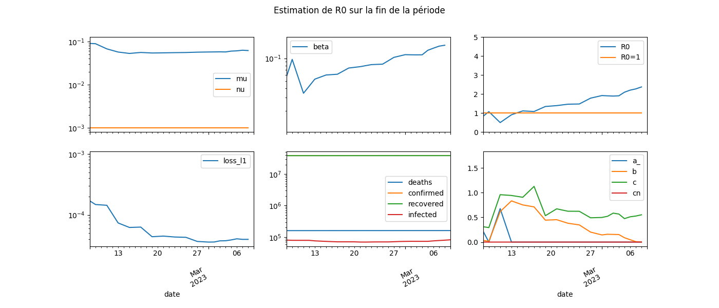
Graphe sur les dernières valeurs.

dfcoeflast = dfcoef.iloc[-30:, :]
dflast = df.iloc[-30:, :]

fig, ax = plt.subplots(2, 3, figsize=(14, 6), sharex=True)
with warnings.catch_warnings():
    warnings.simplefilter("ignore", DeprecationWarning)
    dfcoeflast[["mu", "nu"]].plot(ax=ax[0, 0], logy=True)
    dfcoeflast[["beta"]].plot(ax=ax[0, 1], logy=True)
    dfcoeflast[["loss_l1"]].plot(ax=ax[1, 0], logy=True)
    dfcoeflast[["R0", "R0=1"]].plot(ax=ax[0, 2])
    ax[0, 2].set_ylim(0, 5)
    dfcoeflast[["a_", "b", "c", "cn"]].plot(ax=ax[1, 2])
    dflast.drop('safe', axis=1).plot(ax=ax[1, 1], logy=True)
    for i in range(ax.shape[1]):
        for tick in ax[1, i].get_xticklabels():
            tick.set_rotation(30)
    fig.suptitle('Estimation de R0 sur la fin de la période', fontsize=12)
plt.show()

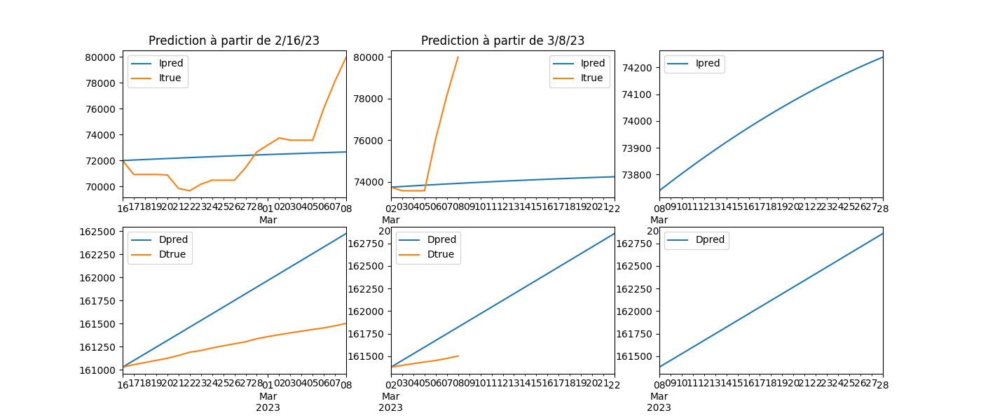
Prédictions

Ce ne sont pas seulement des prédictions mais des prédictions en boucle à partir d’un état initial. On utilise la méthode simulate.

predictions = model.simulate(X[-30:], 21)
df = pandas.DataFrame(
    predictions[9], columns='Spred Ipred Rpred Dpred'.split()).set_index(
        pandas.to_datetime(dates[-21:]))
df.tail()

somewhereaftercovid_39_std/aftercovid/examples/plot_covid_france_sird_cst.py:186: UserWarning: Could not infer format, so each element will be parsed individually, falling back to `dateutil`. To ensure parsing is consistent and as-expected, please specify a format.
  pandas.to_datetime(dates[-21:]))

	Spred	Ipred	Rpred	Dpred
2023-03-04	28394288.0	72548.921875	38345616.0	162184.421875
2023-03-05	28389712.0	72577.304688	38348500.0	162256.984375
2023-03-06	28385136.0	72604.953125	38351384.0	162329.562500
2023-03-07	28380556.0	72631.875000	38354268.0	162402.171875
2023-03-08	28375978.0	72658.070312	38357156.0	162474.812500

On représente les prédictions. Ipred est la valeur prédite, Itrue est la valeur connue. Idem pour Dpred et Dtrue.

fig, ax = plt.subplots(2, 3, figsize=(14, 6))

df = pandas.DataFrame(
    predictions[9], columns='S Ipred R Dpred'.split()).set_index(
        pandas.to_datetime(dates[-21:]))
df[["Ipred"]].plot(ax=ax[0, 0])
df[["Dpred"]].plot(ax=ax[1, 0])
df = pandas.DataFrame(X[-21:], columns='S Itrue R Dtrue'.split()
                      ).set_index(pandas.to_datetime(dates[-21:]))
df[["Itrue"]].plot(ax=ax[0, 0])
df[["Dtrue"]].plot(ax=ax[1, 0])
ax[0, 0].set_title(f"Prediction à partir de {dates[-21]}")

dt = pandas.to_datetime(dates[-7])
dates2 = pandas.to_datetime([dt + timedelta(i) for i in range(21)])
df = pandas.DataFrame(
    predictions[-7], columns='S Ipred R Dpred'.split()).set_index(dates2)
df[["Ipred"]].plot(ax=ax[0, 1])
df[["Dpred"]].plot(ax=ax[1, 1])
df = pandas.DataFrame(X[-7:], columns='S Itrue R Dtrue'.split()
                      ).set_index(pandas.to_datetime(dates[-7:]))
df[["Itrue"]].plot(ax=ax[0, 1])
df[["Dtrue"]].plot(ax=ax[1, 1])
ax[0, 1].set_title(f"Prediction à partir de {dates[-7]}")

dt = pandas.to_datetime(dates[-1])
dates2 = pandas.to_datetime([dt + timedelta(i) for i in range(21)])
df = pandas.DataFrame(
    predictions[-7], columns='S Ipred R Dpred'.split()).set_index(dates2)
df[["Ipred"]].plot(ax=ax[0, 2])
df[["Dpred"]].plot(ax=ax[1, 2])
ax[0, 1].set_title(f"Prediction à partir de {dates[-1]}")
plt.show()

somewhereaftercovid_39_std/aftercovid/examples/plot_covid_france_sird_cst.py:198: UserWarning: Could not infer format, so each element will be parsed individually, falling back to `dateutil`. To ensure parsing is consistent and as-expected, please specify a format.
  pandas.to_datetime(dates[-21:]))
somewhereaftercovid_39_std/aftercovid/examples/plot_covid_france_sird_cst.py:202: UserWarning: Could not infer format, so each element will be parsed individually, falling back to `dateutil`. To ensure parsing is consistent and as-expected, please specify a format.
  ).set_index(pandas.to_datetime(dates[-21:]))
somewhereaftercovid_39_std/aftercovid/examples/plot_covid_france_sird_cst.py:214: UserWarning: Could not infer format, so each element will be parsed individually, falling back to `dateutil`. To ensure parsing is consistent and as-expected, please specify a format.
  ).set_index(pandas.to_datetime(dates[-7:]))

Ces prédictions varient beaucoup car une petite imprécision sur l’estimation a beaucoup d’impact à moyen terme.