Ideas on City Bike Challenge#

Links: notebook, html, PDF, python, slides, GitHub

Based on the data available at Divvy Data, how to guess where people usually live and where the usually work? This notebook suggests some directions and shows some results.

from jyquickhelper import add_notebook_menu
add_notebook_menu()

%matplotlib inline

The data #

Divvy Data publishes a sample of the data.

from pyensae.datasource import download_data
file = download_data("Divvy_Trips_2016_Q3Q4.zip", url="https://s3.amazonaws.com/divvy-data/tripdata/")

We know the stations.

import pandas
stations = df = pandas.read_csv("Divvy_Stations_2016_Q3.csv")
df.head()

	id	name	latitude	longitude	dpcapacity	online_date
0	456	2112 W Peterson Ave	41.991178	-87.683593	15	5/12/2015
1	101	63rd St Beach	41.781016	-87.576120	23	4/20/2015
2	109	900 W Harrison St	41.874675	-87.650019	19	8/6/2013
3	21	Aberdeen St & Jackson Blvd	41.877726	-87.654787	15	6/21/2013
4	80	Aberdeen St & Monroe St	41.880420	-87.655599	19	6/26/2013

And we know the trips.

bikes = df = pandas.read_csv("Divvy_Trips_2016_Q3.csv")
df.head()

	trip_id	starttime	stoptime	bikeid	tripduration	from_station_id	from_station_name	to_station_id	to_station_name	usertype	gender	birthyear
0	12150160	9/30/2016 23:59:58	10/1/2016 00:04:03	4959	245	69	Damen Ave & Pierce Ave	17	Wood St & Division St	Subscriber	Male	1988.0
1	12150159	9/30/2016 23:59:58	10/1/2016 00:04:09	2589	251	383	Ashland Ave & Harrison St	320	Loomis St & Lexington St	Subscriber	Female	1990.0
2	12150158	9/30/2016 23:59:51	10/1/2016 00:24:51	3656	1500	302	Sheffield Ave & Wrightwood Ave	334	Lake Shore Dr & Belmont Ave	Customer	NaN	NaN
3	12150157	9/30/2016 23:59:51	10/1/2016 00:03:56	3570	245	475	Washtenaw Ave & Lawrence Ave	471	Francisco Ave & Foster Ave	Subscriber	Female	1988.0
4	12150156	9/30/2016 23:59:32	10/1/2016 00:26:50	3158	1638	302	Sheffield Ave & Wrightwood Ave	492	Leavitt St & Addison St	Customer	NaN	NaN

First assumption #

Which time do you go to work? How do you go to work? Maybe by bicycles, maybe in the morning, everyday… Let’s see the distribution of the stop time in every station of one particular day of the week.

import pandas
from datetime import datetime, time
df["dtstart"] = pandas.to_datetime(df.starttime, infer_datetime_format=True)
df["dtstop"] = pandas.to_datetime(df.stoptime, infer_datetime_format=True)
df["stopday"] = df.dtstop.apply(lambda r: datetime(r.year, r.month, r.day))
df["stoptime"] = df.dtstop.apply(lambda r: time(r.hour, r.minute, 0))
df["stoptime10"] = df.dtstop.apply(lambda r: time(r.hour, (r.minute // 10)*10, 0))  # every 10 minutes

df['stopweekday'] = df['dtstop'].dt.dayofweek

Big stations #

We average the number of the number of bicycles which stops at the station.

key = ["to_station_name", "to_station_id", "stopday"]
perday = df[key + ["trip_id"]].groupby(key, as_index=False).count()
ave = perday.groupby(key[:-1], as_index=False).mean()
ave.columns = "to_station_name", "to_station_id", "mean stops per day"
ave.head()

	to_station_name	to_station_id	mean stops per day
0	2112 W Peterson Ave	456	2.532468
1	63rd St Beach	101	6.316456
2	900 W Harrison St	109	17.347826
3	Aberdeen St & Jackson Blvd	21	36.402174
4	Aberdeen St & Monroe St	80	40.793478

ax = ave["mean stops per day"].hist(bins=50, figsize=(14,4))
ax.set_xlim([0, 300])
ax.set_yscale("log")
ax.set_title("mean stops per day")
ax.set_xlabel("mean stops per day")
ax.set_ylabel("number of stations");

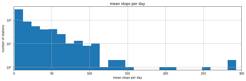
ave[ave["mean stops per day"] > 20].shape, ave.shape

((236, 3), (581, 3))

df.dtstop.min(), df.dtstop.max()

(Timestamp('2016-07-01 00:03:37'), Timestamp('2016-10-01 09:24:02'))

For about half of the stations, more than 20 bicycles stops between July and October of 2016. Let’s take one of them.

ave[ave["mean stops per day"] > 20].head()

	to_station_name	to_station_id	mean stops per day
3	Aberdeen St & Jackson Blvd	21	36.402174
4	Aberdeen St & Monroe St	80	40.793478
5	Ada St & Washington Blvd	346	34.728261
6	Adler Planetarium	341	114.478261
9	Albany Ave & Bloomingdale Ave	511	20.913043

key = ["to_station_name", "to_station_id", "stopweekday", "stoptime10"]
snippet = df[key + ["trip_id"]].groupby(key, as_index=False).count()
snippet.columns = "to_station_name", "to_station_id", "stopweekday", "stoptime10", "nb_stops"
snippet21 = snippet[snippet["to_station_id"] == 21].copy()
snippet21.head()

	to_station_name	to_station_id	stoptime10	nb_stops
925	Aberdeen St & Jackson Blvd	21	05:10:00	4
926	Aberdeen St & Jackson Blvd	21	06:00:00	1
927	Aberdeen St & Jackson Blvd	21	06:10:00	4
928	Aberdeen St & Jackson Blvd	21	06:20:00	2
929	Aberdeen St & Jackson Blvd	21	06:40:00	1

snippet21.tail()

	to_station_name	to_station_id	stopweekday	stoptime10	nb_stops
1621	Aberdeen St & Jackson Blvd	21	6	22:10:00	7
1622	Aberdeen St & Jackson Blvd	21	6	22:20:00	1
1623	Aberdeen St & Jackson Blvd	21	6	22:30:00	2
1624	Aberdeen St & Jackson Blvd	21	6	22:50:00	1
1625	Aberdeen St & Jackson Blvd	21	6	23:40:00	1

from ensae_projects.datainc.data_bikes import add_missing_time
import matplotlib.pyplot as plt
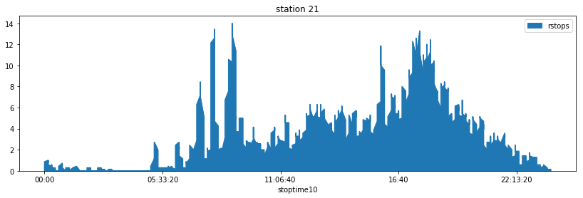
fig, ax = plt.subplots(1,1, figsize=(14,4))
full_snippet21 = add_missing_time(snippet21, "stoptime10", delay=10, values="nb_stops")
full_snippet21["rstops"] = full_snippet21.nb_stops.rolling(7).mean()
full_snippet21.plot(x="stoptime10", y="rstops", figsize=(14,4), kind="area", ax=ax)
ax.set_title("station 21");

from ensae_projects.datainc.data_bikes import add_missing_time
import matplotlib.pyplot as plt
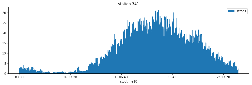
fig, ax = plt.subplots(1,1, figsize=(14,4))
sni = snippet[snippet["to_station_id"] == 341].copy()
sni = add_missing_time(sni, "stoptime10", delay=10, values="nb_stops")
sni["rstops"] = sni.nb_stops.rolling(7).mean()
sni.plot(x="stoptime10", y="rstops", figsize=(14,4), kind="area", ax=ax)
ax.set_title("station 341");

If a station is inside working area, people will arrive in the morning and will leave in the evening. If it is a living area, people should leave in the morning and arrive in the evening. Let’s note $L_t$ the number of bicyles leaving a station. Let’s compute the ratio:

$R = \frac{\sum_{t=8am}^{12am} L_t}{\sum_{t=0am}^{12pm} L_t}$

col = full_snippet21["stoptime10"]
R21 = full_snippet21.nb_stops[(col > time(8,0,0)) & (col < time(12,0,0))].sum() /  \
      full_snippet21.nb_stops[col >= time(0,0,0)].sum()
R21

0.1803523439832786

key = ["to_station_name", "to_station_id", "stopweekday", "stoptime10"]
agg = bikes[key + ["trip_id"]].groupby(key, as_index=False).count().copy()

ratios = {}
for ids in set(stations.id):
    sni = agg[agg["to_station_id"] == ids]
    sni.columns = "to_station_name", "to_station_id", "stopweekday", "stoptime10", "nb_stops"
    num = sni.nb_stops[(sni["stoptime10"] >= time(8,0,0)) & (sni["stoptime10"] <= time(12,0,0))].sum()
    den = sni.nb_stops[sni["stoptime10"] >= time(0,0,0)].sum()
    if den > 0:
        ratios[ids] = num * 1.0 / den

import numpy
stations_ratio = stations.copy()
stations_ratio["ratio"] = stations.id.apply(lambda x: ratios.get(x, numpy.nan))
stations_ratio.head()

	id	name	latitude	longitude	dpcapacity	online_date	ratio
0	456	2112 W Peterson Ave	41.991178	-87.683593	15	5/12/2015	0.102564
1	101	63rd St Beach	41.781016	-87.576120	23	4/20/2015	0.254509
2	109	900 W Harrison St	41.874675	-87.650019	19	8/6/2013	0.392231
3	21	Aberdeen St & Jackson Blvd	41.877726	-87.654787	15	6/21/2013	0.196178
4	80	Aberdeen St & Monroe St	41.880420	-87.655599	19	6/26/2013	0.192379

stations_ratio["ratio"].hist(bins=50);

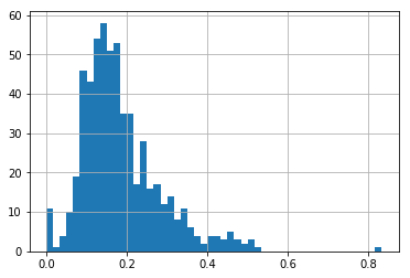
We choose the median.

stations_ratio.ratio.median()

0.1648655139289145

And we draw a map.

from ensae_projects.datainc.data_bikes import folium_html_stations_map
xy = []
for els in stations_ratio.apply(lambda row: (row["latitude"], row["longitude"], row["ratio"], row["name"]), axis=1):
    name = "%s %1.2f" % (els[3], els[2])
    color = "red" if els[2] >= 0.1648655139289145 else "blue"
    xy.append( ( (els[0], els[1]), (name, color)))
folium_html_stations_map(xy, width="80%")

If we assume that people have bigger flats than working space, we should assume there are more living areas than working areas.

stations_ratio.ratio.quantile(0.6)

0.18241042345276873

from ensae_projects.datainc.data_bikes import folium_html_stations_map
xy = []
for els in stations_ratio.apply(lambda row: (row["latitude"], row["longitude"], row["ratio"], row["name"]), axis=1):
    name = "%s %1.2f" % (els[3], els[2])
    color = "red" if els[2] >= 0.18241042345276873 else "blue"
    xy.append( ( (els[0], els[1]), (name, color)))
folium_html_stations_map(xy, width="80%")

Links

Contents

Information

Previous topic

Next topic

Ideas on City Bike Challenge#

The data #

First assumption #

Big stations #

Indicator #

Links

Contents

Information

Previous topic

Next topic

Ideas on City Bike Challenge#

The data#

First assumption#

Big stations#

Indicator#

The data #

First assumption #

Big stations #

Indicator #