Bike Pattern#
Links: notebook, html, PDF, python, slides, GitHub
We used a little bit of machine learning on Divvy Data to dig into a better division of Chicago. We try to identify patterns among bike stations.
from jyquickhelper import add_notebook_menu
add_notebook_menu()
%matplotlib inline
The data#
Divvy Data publishes a sample of the data.
from pyensae.datasource import download_data
file = download_data("Divvy_Trips_2016_Q3Q4.zip", url="https://s3.amazonaws.com/divvy-data/tripdata/")
We know the stations.
import pandas
stations = pandas.read_csv("Divvy_Stations_2016_Q3.csv")
bikes = pandas.concat([pandas.read_csv("Divvy_Trips_2016_Q3.csv"),
                       pandas.read_csv("Divvy_Trips_2016_Q4.csv")])
from datetime import datetime, time
df = bikes
df["dtstart"] = pandas.to_datetime(df.starttime, infer_datetime_format=True)
df["dtstop"] = pandas.to_datetime(df.stoptime, infer_datetime_format=True)
df["stopday"] = df.dtstop.apply(lambda r: datetime(r.year, r.month, r.day))
df["stoptime"] = df.dtstop.apply(lambda r: time(r.hour, r.minute, 0))
df["stoptime10"] = df.dtstop.apply(lambda r: time(r.hour, (r.minute // 10)*10, 0))  # every 10 minutes
df['stopweekday'] = df['dtstop'].dt.dayofweek
Normalize per week day (stop)#
df.columns
Index(['trip_id', 'starttime', 'stoptime', 'bikeid', 'tripduration',
       'from_station_id', 'from_station_name', 'to_station_id',
       'to_station_name', 'usertype', 'gender', 'birthyear', 'dtstart',
       'dtstop', 'stopday', 'stoptime10', 'stopweekday'],
      dtype='object')
key = ["to_station_id", "to_station_name", "stopweekday", "stoptime10"]
keep = key + ["trip_id"]
aggtime = df[keep].groupby(key, as_index=False).count()
aggtime.columns = key + ["nb_trips"]
aggtime.head()
| to_station_id | to_station_name | stopweekday | stoptime10 | nb_trips | |
|---|---|---|---|---|---|
| 0 | 2 | Michigan Ave & Balbo Ave | 0 | 00:10:00 | 2 |
| 1 | 2 | Michigan Ave & Balbo Ave | 0 | 00:20:00 | 2 |
| 2 | 2 | Michigan Ave & Balbo Ave | 0 | 00:30:00 | 2 |
| 3 | 2 | Michigan Ave & Balbo Ave | 0 | 01:00:00 | 3 |
| 4 | 2 | Michigan Ave & Balbo Ave | 0 | 01:10:00 | 2 |
aggday = df[keep[:-2] + ["trip_id"]].groupby(key[:-1], as_index=False).count()
aggday.columns = key[:-1] + ["nb_trips"]
aggday.sort_values("nb_trips", ascending=False).head()
| to_station_id | to_station_name | stopweekday | nb_trips | |
|---|---|---|---|---|
| 222 | 35 | Streeter Dr & Grand Ave | 5 | 15380 |
| 223 | 35 | Streeter Dr & Grand Ave | 6 | 14680 |
| 217 | 35 | Streeter Dr & Grand Ave | 0 | 9228 |
| 221 | 35 | Streeter Dr & Grand Ave | 4 | 7945 |
| 1741 | 268 | Lake Shore Dr & North Blvd | 5 | 7508 |
merge = aggtime.merge(aggday, on=key[:-1], suffixes=("", "day"))
merge.head()
| to_station_id | to_station_name | stopweekday | stoptime10 | nb_trips | nb_tripsday | |
|---|---|---|---|---|---|---|
| 0 | 2 | Michigan Ave & Balbo Ave | 0 | 00:10:00 | 2 | 913 |
| 1 | 2 | Michigan Ave & Balbo Ave | 0 | 00:20:00 | 2 | 913 |
| 2 | 2 | Michigan Ave & Balbo Ave | 0 | 00:30:00 | 2 | 913 |
| 3 | 2 | Michigan Ave & Balbo Ave | 0 | 01:00:00 | 3 | 913 |
| 4 | 2 | Michigan Ave & Balbo Ave | 0 | 01:10:00 | 2 | 913 |
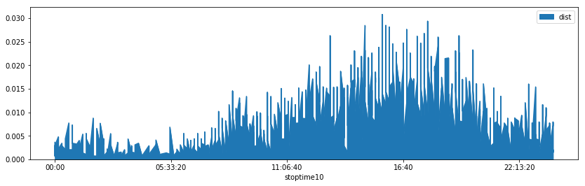
merge["dist"] = merge["nb_trips"] / merge["nb_tripsday"]
merge.head()
| to_station_id | to_station_name | stopweekday | stoptime10 | nb_trips | nb_tripsday | dist | |
|---|---|---|---|---|---|---|---|
| 0 | 2 | Michigan Ave & Balbo Ave | 0 | 00:10:00 | 2 | 913 | 0.002191 |
| 1 | 2 | Michigan Ave & Balbo Ave | 0 | 00:20:00 | 2 | 913 | 0.002191 |
| 2 | 2 | Michigan Ave & Balbo Ave | 0 | 00:30:00 | 2 | 913 | 0.002191 |
| 3 | 2 | Michigan Ave & Balbo Ave | 0 | 01:00:00 | 3 | 913 | 0.003286 |
| 4 | 2 | Michigan Ave & Balbo Ave | 0 | 01:10:00 | 2 | 913 | 0.002191 |
merge[merge["to_station_id"] == 2].plot(x="stoptime10", y="dist", figsize=(14,4), kind="area");
Clustering (stop)#
We cluster these distribution to find some patterns. But we need vectors of equal size which should be equal to 24*6.
print(key)
merge.groupby(key[:-1], as_index=False).count().head()
['to_station_id', 'to_station_name', 'stopweekday', 'stoptime10']
| to_station_id | to_station_name | stopweekday | stoptime10 | nb_trips | nb_tripsday | dist | |
|---|---|---|---|---|---|---|---|
| 0 | 2 | Michigan Ave & Balbo Ave | 0 | 114 | 114 | 114 | 114 |
| 1 | 2 | Michigan Ave & Balbo Ave | 1 | 109 | 109 | 109 | 109 |
| 2 | 2 | Michigan Ave & Balbo Ave | 2 | 116 | 116 | 116 | 116 |
| 3 | 2 | Michigan Ave & Balbo Ave | 3 | 112 | 112 | 112 | 112 |
| 4 | 2 | Michigan Ave & Balbo Ave | 4 | 117 | 117 | 117 | 117 |
from ensae_projects.datainc.data_bikes import add_missing_time
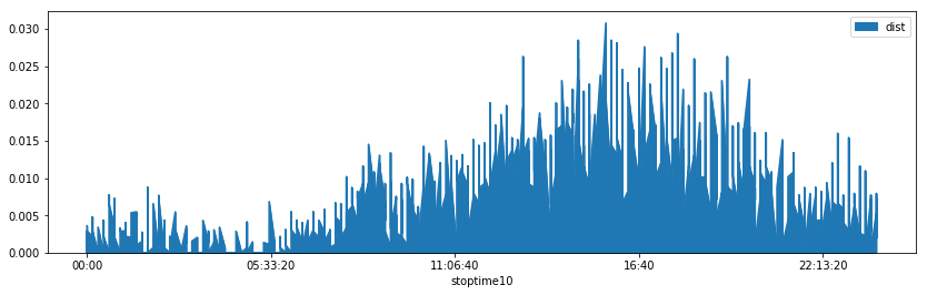
full = df = add_missing_time(merge, delay=10, column="stoptime10", values=["nb_trips", "nb_tripsday", "dist"])
df.groupby(key[:-1], as_index=False).count().head()
| to_station_id | to_station_name | stopweekday | stoptime10 | nb_trips | nb_tripsday | dist | |
|---|---|---|---|---|---|---|---|
| 0 | 2 | Michigan Ave & Balbo Ave | 0 | 144 | 144 | 144 | 144 |
| 1 | 2 | Michigan Ave & Balbo Ave | 1 | 144 | 144 | 144 | 144 |
| 2 | 2 | Michigan Ave & Balbo Ave | 2 | 144 | 144 | 144 | 144 |
| 3 | 2 | Michigan Ave & Balbo Ave | 3 | 144 | 144 | 144 | 144 |
| 4 | 2 | Michigan Ave & Balbo Ave | 4 | 144 | 144 | 144 | 144 |
This is much better.
df[df["to_station_id"] == 2].plot(x="stoptime10", y="dist", figsize=(14,4), kind="area");
Let’s build the features.
features = df.pivot_table(index=["to_station_id", "to_station_name", "stopweekday"],
                          columns="stoptime10", values="dist").reset_index()
features.head()
| stoptime10 | to_station_id | to_station_name | stopweekday | 00:00:00 | 00:10:00 | 00:20:00 | 00:30:00 | 00:40:00 | 00:50:00 | 01:00:00 | ... | 22:20:00 | 22:30:00 | 22:40:00 | 22:50:00 | 23:00:00 | 23:10:00 | 23:20:00 | 23:30:00 | 23:40:00 | 23:50:00 |
|---|---|---|---|---|---|---|---|---|---|---|---|---|---|---|---|---|---|---|---|---|---|
| 0 | 2 | Michigan Ave & Balbo Ave | 0 | 0.000000 | 0.002191 | 0.002191 | 0.002191 | 0.000000 | 0.000000 | 0.003286 | ... | 0.004381 | 0.002191 | 0.004381 | 0.002191 | 0.004381 | 0.004381 | 0.005476 | 0.002191 | 0.000000 | 0.005476 |
| 1 | 2 | Michigan Ave & Balbo Ave | 1 | 0.000000 | 0.002677 | 0.000000 | 0.000000 | 0.001339 | 0.002677 | 0.000000 | ... | 0.009371 | 0.012048 | 0.006693 | 0.004016 | 0.005355 | 0.006693 | 0.002677 | 0.000000 | 0.000000 | 0.000000 |
| 2 | 2 | Michigan Ave & Balbo Ave | 2 | 0.002907 | 0.002907 | 0.002907 | 0.004360 | 0.001453 | 0.007267 | 0.002907 | ... | 0.002907 | 0.002907 | 0.015988 | 0.005814 | 0.001453 | 0.001453 | 0.011628 | 0.000000 | 0.000000 | 0.007267 |
| 3 | 2 | Michigan Ave & Balbo Ave | 3 | 0.000000 | 0.000000 | 0.000000 | 0.000000 | 0.007728 | 0.000000 | 0.001546 | ... | 0.009274 | 0.003091 | 0.003091 | 0.007728 | 0.001546 | 0.003091 | 0.009274 | 0.001546 | 0.007728 | 0.001546 |
| 4 | 2 | Michigan Ave & Balbo Ave | 4 | 0.002053 | 0.000000 | 0.000000 | 0.002053 | 0.000000 | 0.002053 | 0.003080 | ... | 0.008214 | 0.001027 | 0.006160 | 0.004107 | 0.015400 | 0.006160 | 0.002053 | 0.006160 | 0.007187 | 0.000000 |
5 rows × 147 columns
names = features.columns[3:]
names
Index([00:00:00, 00:10:00, 00:20:00, 00:30:00, 00:40:00, 00:50:00, 01:00:00,
       01:10:00, 01:20:00, 01:30:00,
       ...
       22:20:00, 22:30:00, 22:40:00, 22:50:00, 23:00:00, 23:10:00, 23:20:00,
       23:30:00, 23:40:00, 23:50:00],
      dtype='object', name='stoptime10', length=144)
from sklearn.cluster import KMeans
clus = KMeans(8)
clus.fit(features[names])
KMeans(algorithm='auto', copy_x=True, init='k-means++', max_iter=300,
    n_clusters=8, n_init=10, n_jobs=1, precompute_distances='auto',
    random_state=None, tol=0.0001, verbose=0)
pred = clus.predict(features[names])
set(pred)
{0, 1, 2, 3, 4, 5, 6, 7}
features["cluster"] = pred
Let’s see what it means accross day.
features[["cluster", "stopweekday", "to_station_id"]].groupby(["cluster", "stopweekday"]).count()
| stoptime10 | to_station_id | |
|---|---|---|
| cluster | stopweekday | |
| 0 | 0 | 304 |
| 1 | 348 | |
| 2 | 337 | |
| 3 | 315 | |
| 4 | 275 | |
| 5 | 36 | |
| 6 | 46 | |
| 1 | 0 | 2 |
| 1 | 1 | |
| 2 | 1 | |
| 6 | 1 | |
| 2 | 5 | 2 |
| 3 | 0 | 1 |
| 2 | 1 | |
| 3 | 1 | |
| 4 | 2 | |
| 4 | 0 | 1 |
| 1 | 1 | |
| 2 | 1 | |
| 3 | 1 | |
| 5 | 0 | 1 |
| 6 | 2 | |
| 6 | 0 | 123 |
| 1 | 133 | |
| 2 | 143 | |
| 3 | 137 | |
| 4 | 147 | |
| 5 | 13 | |
| 6 | 11 | |
| 7 | 0 | 141 |
| 1 | 93 | |
| 2 | 94 | |
| 3 | 121 | |
| 4 | 154 | |
| 5 | 526 | |
| 6 | 514 |
Let’s draw the clusters.
centers = clus.cluster_centers_.T
import matplotlib.pyplot as plt
fig, ax = plt.subplots(centers.shape[1], 1, figsize=(10,10))
x = list(range(0,centers.shape[0]))
for i in range(centers.shape[1]):
    ax[i].bar (x, centers[:,i], width=1.0)
    ax[i].set_ylabel("cluster %d" % i)
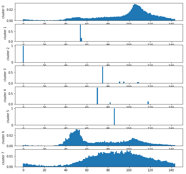
Three patterns emerge. However, small clusters are still annoying but let’s show them on a map.
Graph#
We first need to get 7 clusters for each stations, one per day.
piv = features.pivot_table(index=["to_station_id","to_station_name"], columns="stopweekday", values="cluster")
piv.head()
| stopweekday | 0 | 1 | 2 | 3 | 4 | 5 | 6 | |
|---|---|---|---|---|---|---|---|---|
| to_station_id | to_station_name | |||||||
| 2 | Michigan Ave & Balbo Ave | 7.0 | 0.0 | 7.0 | 7.0 | 7.0 | 7.0 | 7.0 |
| 3 | Shedd Aquarium | 7.0 | 7.0 | 7.0 | 7.0 | 7.0 | 7.0 | 7.0 |
| 4 | Burnham Harbor | 7.0 | 7.0 | 0.0 | 7.0 | 7.0 | 7.0 | 7.0 |
| 5 | State St & Harrison St | 0.0 | 0.0 | 0.0 | 0.0 | 0.0 | 7.0 | 7.0 |
| 6 | Dusable Harbor | 7.0 | 7.0 | 0.0 | 7.0 | 7.0 | 7.0 | 7.0 |
piv["distincts"] = piv.apply(lambda row: len(set(row[i] for i in range(0,7))), axis=1)
Let’s see which station is classified in more than 4 clusters. NaN means no bikes stopped at this stations. They are mostly unused stations.
piv[piv.distincts >= 4]
| stopweekday | 0 | 1 | 2 | 3 | 4 | 5 | 6 | distincts | |
|---|---|---|---|---|---|---|---|---|---|
| to_station_id | to_station_name | ||||||||
| 384 | Halsted St & 51st St | NaN | 7.0 | 7.0 | 7.0 | 0.0 | 0.0 | 6.0 | 4 |
| 386 | Halsted St & 56th St | 5.0 | 7.0 | 0.0 | 7.0 | 7.0 | 7.0 | 6.0 | 4 |
| 409 | Shields Ave & 43rd St | 7.0 | NaN | 7.0 | NaN | 6.0 | 0.0 | 7.0 | 5 |
| 530 | Laramie Ave & Kinzie St | 3.0 | 7.0 | 7.0 | 7.0 | 0.0 | 6.0 | 7.0 | 4 |
| 538 | Cicero Ave & Flournoy St | 7.0 | 6.0 | NaN | 6.0 | 7.0 | 7.0 | 5.0 | 4 |
| 543 | Laramie Ave & Gladys Ave | 0.0 | 7.0 | 6.0 | 6.0 | 6.0 | 6.0 | NaN | 4 |
| 548 | Morgan St & Pershing Rd | NaN | 7.0 | 7.0 | 6.0 | 0.0 | 7.0 | 0.0 | 4 |
| 556 | Throop St & 52nd St | 7.0 | 0.0 | 7.0 | 3.0 | 0.0 | 2.0 | 7.0 | 4 |
| 557 | Damen Ave & Garfield Blvd | NaN | 0.0 | 3.0 | NaN | NaN | NaN | NaN | 7 |
| 558 | Ashland Ave & Garfield Blvd | NaN | 7.0 | 7.0 | 0.0 | 3.0 | 7.0 | NaN | 5 |
| 561 | Damen Ave & 61st St | 1.0 | 6.0 | 6.0 | 0.0 | NaN | 7.0 | 7.0 | 5 |
| 562 | Racine Ave & 61st St | NaN | NaN | NaN | NaN | 6.0 | NaN | NaN | 7 |
| 564 | Racine Ave & 65th St | 7.0 | NaN | NaN | NaN | 0.0 | 2.0 | 6.0 | 7 |
| 565 | Ashland Ave & 66th St | 7.0 | 0.0 | NaN | 7.0 | 7.0 | NaN | 0.0 | 4 |
| 567 | May St & 69th St | 1.0 | 1.0 | 6.0 | 6.0 | 6.0 | NaN | NaN | 4 |
| 569 | Woodlawn Ave & 75th St | NaN | NaN | 0.0 | 7.0 | 0.0 | NaN | NaN | 6 |
| 576 | Greenwood Ave & 79th St | 0.0 | 0.0 | 0.0 | NaN | 6.0 | NaN | 0.0 | 4 |
| 580 | Exchange Ave & 79th St | 4.0 | NaN | 0.0 | 0.0 | 0.0 | 7.0 | 0.0 | 4 |
| 581 | Commercial Ave & 83rd St | 7.0 | NaN | 0.0 | NaN | NaN | 7.0 | 0.0 | 5 |
| 582 | Phillips Ave & 82nd St | NaN | NaN | 7.0 | 7.0 | NaN | 7.0 | 0.0 | 5 |
| 584 | Ellis Ave & 83rd St | NaN | 7.0 | NaN | 6.0 | 6.0 | 7.0 | NaN | 5 |
| 586 | MLK Jr Dr & 83rd St | 7.0 | 6.0 | 1.0 | 6.0 | 6.0 | 0.0 | 0.0 | 4 |
| 587 | Wabash Ave & 83rd St | NaN | NaN | 7.0 | NaN | 7.0 | 6.0 | 0.0 | 6 |
| 588 | South Chicago Ave & 83rd St | NaN | 0.0 | 0.0 | NaN | 7.0 | 7.0 | 0.0 | 4 |
| 591 | Kilbourn Ave & Milwaukee Ave | 0.0 | 6.0 | 6.0 | 6.0 | 6.0 | 7.0 | NaN | 4 |
| 593 | Halsted St & 59th St | NaN | 4.0 | 7.0 | 7.0 | NaN | 7.0 | 5.0 | 5 |
Let’s draw a map on a week day.
data = stations.merge(piv.reset_index(), left_on=["id", "name"],
                      right_on=["to_station_id", "to_station_name"], suffixes=('', '_c'))
data.sort_values("id").head()
| id | name | latitude | longitude | dpcapacity | online_date | to_station_id | to_station_name | 0 | 1 | 2 | 3 | 4 | 5 | 6 | distincts | |
|---|---|---|---|---|---|---|---|---|---|---|---|---|---|---|---|---|
| 357 | 2 | Michigan Ave & Balbo Ave | 41.872638 | -87.623979 | 35 | 5/8/2015 | 2 | Michigan Ave & Balbo Ave | 7.0 | 0.0 | 7.0 | 7.0 | 7.0 | 7.0 | 7.0 | 2 |
| 456 | 3 | Shedd Aquarium | 41.867226 | -87.615355 | 31 | 4/24/2015 | 3 | Shedd Aquarium | 7.0 | 7.0 | 7.0 | 7.0 | 7.0 | 7.0 | 7.0 | 1 |
| 53 | 4 | Burnham Harbor | 41.856268 | -87.613348 | 23 | 5/16/2015 | 4 | Burnham Harbor | 7.0 | 7.0 | 0.0 | 7.0 | 7.0 | 7.0 | 7.0 | 2 |
| 497 | 5 | State St & Harrison St | 41.874053 | -87.627716 | 23 | 6/18/2013 | 5 | State St & Harrison St | 0.0 | 0.0 | 0.0 | 0.0 | 0.0 | 7.0 | 7.0 | 2 |
| 188 | 6 | Dusable Harbor | 41.885042 | -87.612795 | 31 | 4/24/2015 | 6 | Dusable Harbor | 7.0 | 7.0 | 0.0 | 7.0 | 7.0 | 7.0 | 7.0 | 2 |
from ensae_projects.datainc.data_bikes import folium_html_stations_map

colors = ["blue", "red", "yellow", "gray", "green", "black", "brown"]
xy = []
for els in data.apply(lambda row: (row["latitude"], row["longitude"], row[1], row["name"]), axis=1):
    try:
        cl = int(els[2])
    except:
        # NaN
        continue
    name = "%s c%d" % (els[3], cl)
    color = colors[cl % len(colors)]
    xy.append( ( (els[0], els[1]), (name, color)))
folium_html_stations_map(xy, width="80%")
We notice than people got to the park after work. Let’s see during the week-end.
from ensae_projects.datainc.data_bikes import folium_html_stations_map

colors = ["blue", "red", "yellow", "gray", "green", "black", "brown"]
xy = []
for els in data.apply(lambda row: (row["latitude"], row["longitude"], row[5], row["name"]), axis=1):
    try:
        cl = int(els[2])
    except:
        # NaN
        continue
    name = "%s c%d" % (els[3], cl)
    color = colors[cl % len(colors)]
    xy.append( ( (els[0], els[1]), (name, color)))
folium_html_stations_map(xy, width="80%")