Bike Pattern 2#
Links: notebook, html, PDF, python, slides, GitHub
We used a little bit of machine learning on Divvy Data to dig into a better division of Chicago. We try to identify patterns among bike stations.
from jyquickhelper import add_notebook_menu
add_notebook_menu()
%matplotlib inline
The data#
Divvy Data publishes a sample of the data.
from pyensae.datasource import download_data
file = download_data("Divvy_Trips_2016_Q3Q4.zip", url="https://s3.amazonaws.com/divvy-data/tripdata/")
We know the stations.
import pandas
stations = pandas.read_csv("Divvy_Stations_2016_Q3.csv")
bikes = pandas.concat([pandas.read_csv("Divvy_Trips_2016_Q3.csv"),
                       pandas.read_csv("Divvy_Trips_2016_Q4.csv")])
bikes.head()
| trip_id | starttime | stoptime | bikeid | tripduration | from_station_id | from_station_name | to_station_id | to_station_name | usertype | gender | birthyear | |
|---|---|---|---|---|---|---|---|---|---|---|---|---|
| 0 | 12150160 | 9/30/2016 23:59:58 | 10/1/2016 00:04:03 | 4959 | 245 | 69 | Damen Ave & Pierce Ave | 17 | Wood St & Division St | Subscriber | Male | 1988.0 |
| 1 | 12150159 | 9/30/2016 23:59:58 | 10/1/2016 00:04:09 | 2589 | 251 | 383 | Ashland Ave & Harrison St | 320 | Loomis St & Lexington St | Subscriber | Female | 1990.0 |
| 2 | 12150158 | 9/30/2016 23:59:51 | 10/1/2016 00:24:51 | 3656 | 1500 | 302 | Sheffield Ave & Wrightwood Ave | 334 | Lake Shore Dr & Belmont Ave | Customer | NaN | NaN |
| 3 | 12150157 | 9/30/2016 23:59:51 | 10/1/2016 00:03:56 | 3570 | 245 | 475 | Washtenaw Ave & Lawrence Ave | 471 | Francisco Ave & Foster Ave | Subscriber | Female | 1988.0 |
| 4 | 12150156 | 9/30/2016 23:59:32 | 10/1/2016 00:26:50 | 3158 | 1638 | 302 | Sheffield Ave & Wrightwood Ave | 492 | Leavitt St & Addison St | Customer | NaN | NaN |
from datetime import datetime, time
df = bikes
df["dtstart"] = pandas.to_datetime(df.starttime, infer_datetime_format=True)
df["dtstop"] = pandas.to_datetime(df.stoptime, infer_datetime_format=True)

df["stopday"] = df.dtstop.apply(lambda r: datetime(r.year, r.month, r.day))
df["stoptime"] = df.dtstop.apply(lambda r: time(r.hour, r.minute, 0))
df["stoptime10"] = df.dtstop.apply(lambda r: time(r.hour, (r.minute // 10)*10, 0))  # every 10 minutes

df["startday"] = df.dtstart.apply(lambda r: datetime(r.year, r.month, r.day))
df["starttime"] = df.dtstart.apply(lambda r: time(r.hour, r.minute, 0))
df["starttime10"] = df.dtstart.apply(lambda r: time(r.hour, (r.minute // 10)*10, 0))  # every 10 minutes
df['stopweekday'] = df['dtstop'].dt.dayofweek
df['startweekday'] = df['dtstart'].dt.dayofweek
Normalize, aggregating and merging per start and stop time#
key = ["to_station_id", "to_station_name", "stopweekday", "stoptime10"]
keep = key + ["trip_id"]

stopaggtime = df[keep].groupby(key, as_index=False).count()
stopaggtime.columns = key + ["nb_trips"]

stopaggday = df[keep[:-2] + ["trip_id"]].groupby(key[:-1], as_index=False).count()
stopaggday.columns = key[:-1] + ["nb_trips"]

stopaggday = df[keep[:-2] + ["trip_id"]].groupby(key[:-1], as_index=False).count()
stopaggday.columns = key[:-1] + ["nb_trips"]

stopmerge = stopaggtime.merge(stopaggday, on=key[:-1], suffixes=("", "day"))
stopmerge["stopdist"] = stopmerge["nb_trips"] / stopmerge["nb_tripsday"]
stopmerge.head()
| to_station_id | to_station_name | stopweekday | stoptime10 | nb_trips | nb_tripsday | stopdist | |
|---|---|---|---|---|---|---|---|
| 0 | 2 | Michigan Ave & Balbo Ave | 0 | 00:10:00 | 2 | 913 | 0.002191 |
| 1 | 2 | Michigan Ave & Balbo Ave | 0 | 00:20:00 | 2 | 913 | 0.002191 |
| 2 | 2 | Michigan Ave & Balbo Ave | 0 | 00:30:00 | 2 | 913 | 0.002191 |
| 3 | 2 | Michigan Ave & Balbo Ave | 0 | 01:00:00 | 3 | 913 | 0.003286 |
| 4 | 2 | Michigan Ave & Balbo Ave | 0 | 01:10:00 | 2 | 913 | 0.002191 |
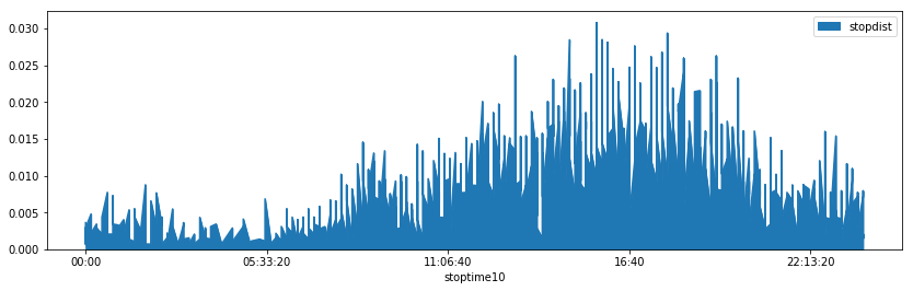
stopmerge[stopmerge["to_station_id"] == 2] \
       .plot(x="stoptime10", y="stopdist", figsize=(14,4), kind="area");
key = ["from_station_id", "from_station_name", "startweekday", "starttime10"]
keep = key + ["trip_id"]

startaggtime = df[keep].groupby(key, as_index=False).count()
startaggtime.columns = key + ["nb_trips"]

startaggday = df[keep[:-2] + ["trip_id"]].groupby(key[:-1], as_index=False).count()
startaggday.columns = key[:-1] + ["nb_trips"]

startaggday = df[keep[:-2] + ["trip_id"]].groupby(key[:-1], as_index=False).count()
startaggday.columns = key[:-1] + ["nb_trips"]

startmerge = startaggtime.merge(startaggday, on=key[:-1], suffixes=("", "day"))
startmerge["startdist"] = startmerge["nb_trips"] / startmerge["nb_tripsday"]
startmerge.head()
| from_station_id | from_station_name | startweekday | starttime10 | nb_trips | nb_tripsday | startdist | |
|---|---|---|---|---|---|---|---|
| 0 | 2 | Michigan Ave & Balbo Ave | 0 | 00:00:00 | 4 | 1065 | 0.003756 |
| 1 | 2 | Michigan Ave & Balbo Ave | 0 | 00:10:00 | 1 | 1065 | 0.000939 |
| 2 | 2 | Michigan Ave & Balbo Ave | 0 | 00:20:00 | 3 | 1065 | 0.002817 |
| 3 | 2 | Michigan Ave & Balbo Ave | 0 | 00:50:00 | 4 | 1065 | 0.003756 |
| 4 | 2 | Michigan Ave & Balbo Ave | 0 | 01:10:00 | 3 | 1065 | 0.002817 |
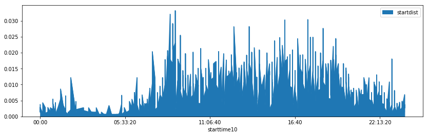
startmerge[startmerge["from_station_id"] == 2] \
         .plot(x="starttime10",  y="startdist", figsize=(14,4), kind="area");
everything = stopmerge.merge(startmerge,
                             left_on=["to_station_id", "to_station_name", "stopweekday", "stoptime10"],
                             right_on=["from_station_id", "from_station_name","startweekday", "starttime10"],
                             suffixes=("stop", "start"),
                             how="outer")
everything.head()
| to_station_id | to_station_name | stopweekday | stoptime10 | nb_tripsstop | nb_tripsdaystop | stopdist | from_station_id | from_station_name | startweekday | starttime10 | nb_tripsstart | nb_tripsdaystart | startdist | |
|---|---|---|---|---|---|---|---|---|---|---|---|---|---|---|
| 0 | 2.0 | Michigan Ave & Balbo Ave | 0.0 | 00:10:00 | 2.0 | 913.0 | 0.002191 | 2.0 | Michigan Ave & Balbo Ave | 0.0 | 00:10:00 | 1.0 | 1065.0 | 0.000939 |
| 1 | 2.0 | Michigan Ave & Balbo Ave | 0.0 | 00:20:00 | 2.0 | 913.0 | 0.002191 | 2.0 | Michigan Ave & Balbo Ave | 0.0 | 00:20:00 | 3.0 | 1065.0 | 0.002817 |
| 2 | 2.0 | Michigan Ave & Balbo Ave | 0.0 | 00:30:00 | 2.0 | 913.0 | 0.002191 | NaN | NaN | NaN | NaN | NaN | NaN | NaN |
| 3 | 2.0 | Michigan Ave & Balbo Ave | 0.0 | 01:00:00 | 3.0 | 913.0 | 0.003286 | NaN | NaN | NaN | NaN | NaN | NaN | NaN |
| 4 | 2.0 | Michigan Ave & Balbo Ave | 0.0 | 01:10:00 | 2.0 | 913.0 | 0.002191 | 2.0 | Michigan Ave & Balbo Ave | 0.0 | 01:10:00 | 3.0 | 1065.0 | 0.002817 |
import numpy
from datetime import datetime

def bestof(x, y):
    if isinstance(x, (datetime, time, str)):
        return x
    try:
        if x is None or isinstance(y, (datetime, time, str)) or numpy.isnan(x):
            return y
        else:
            return x
    except:
        print(type(x), type(y))
        print(x, y)
        raise

bestof(datetime(2017,2,2), numpy.nan), bestof(numpy.nan, datetime(2017,2,2))
(datetime.datetime(2017, 2, 2, 0, 0), datetime.datetime(2017, 2, 2, 0, 0))
every = everything.copy()
every["station_name"] = every.apply(lambda row: bestof(row["to_station_name"], row["from_station_name"]), axis=1)
every["station_id"] = every.apply(lambda row: bestof(row["to_station_id"], row["from_station_id"]), axis=1)
every["time10"] = every.apply(lambda row: bestof(row["stoptime10"], row["starttime10"]), axis=1)
every["weekday"] = every.apply(lambda row: bestof(row["stopweekday"], row["startweekday"]), axis=1)
every = every.drop(["stoptime10", "starttime10", "stopweekday", "startweekday",
                    "to_station_id", "from_station_id",
                    "to_station_name", "from_station_name"], axis=1)
every.head()
| nb_tripsstop | nb_tripsdaystop | stopdist | nb_tripsstart | nb_tripsdaystart | startdist | station_name | station_id | time10 | weekday | |
|---|---|---|---|---|---|---|---|---|---|---|
| 0 | 2.0 | 913.0 | 0.002191 | 1.0 | 1065.0 | 0.000939 | Michigan Ave & Balbo Ave | 2.0 | 00:10:00 | 0.0 |
| 1 | 2.0 | 913.0 | 0.002191 | 3.0 | 1065.0 | 0.002817 | Michigan Ave & Balbo Ave | 2.0 | 00:20:00 | 0.0 |
| 2 | 2.0 | 913.0 | 0.002191 | NaN | NaN | NaN | Michigan Ave & Balbo Ave | 2.0 | 00:30:00 | 0.0 |
| 3 | 3.0 | 913.0 | 0.003286 | NaN | NaN | NaN | Michigan Ave & Balbo Ave | 2.0 | 01:00:00 | 0.0 |
| 4 | 2.0 | 913.0 | 0.002191 | 3.0 | 1065.0 | 0.002817 | Michigan Ave & Balbo Ave | 2.0 | 01:10:00 | 0.0 |
every.shape, stopmerge.shape, startmerge.shape
((357809, 10), (298013, 7), (299700, 7))
We need vectors of equal size which means filling NaN values with 0 and adding times when not present.
every.columns
Index(['nb_tripsstop', 'nb_tripsdaystop', 'stopdist', 'nb_tripsstart',
       'nb_tripsdaystart', 'startdist', 'station_name', 'station_id', 'time10',
       'weekday'],
      dtype='object')
keys = ['station_name', 'station_id', 'weekday', 'time10']
for c in every.columns:
    if c not in keys:
        every[c].fillna(0)
from ensae_projects.datainc.data_bikes import add_missing_time
full = df = add_missing_time(every, delay=10,  column="time10",
                             values=[c for c in every.columns if c not in keys])
full = full[['station_name', 'station_id', 'time10', 'weekday',
             'stopdist', 'startdist',
             'nb_tripsstop', 'nb_tripsdaystop', 'nb_tripsstart',
       'nb_tripsdaystart']].sort_values(keys)
full.head()
| station_name | station_id | time10 | weekday | stopdist | startdist | nb_tripsstop | nb_tripsdaystop | nb_tripsstart | nb_tripsdaystart | |
|---|---|---|---|---|---|---|---|---|---|---|
| 357809 | 2112 W Peterson Ave | 456.0 | 00:00:00 | 0.0 | 0.0 | 0.000000 | 0.0 | 0.0 | 0.0 | 0.0 |
| 357810 | 2112 W Peterson Ave | 456.0 | 00:10:00 | 0.0 | 0.0 | 0.000000 | 0.0 | 0.0 | 0.0 | 0.0 |
| 357811 | 2112 W Peterson Ave | 456.0 | 00:20:00 | 0.0 | 0.0 | 0.000000 | 0.0 | 0.0 | 0.0 | 0.0 |
| 341443 | 2112 W Peterson Ave | 456.0 | 00:30:00 | 0.0 | 0.0 | 0.021277 | 0.0 | 0.0 | 1.0 | 47.0 |
| 357812 | 2112 W Peterson Ave | 456.0 | 00:40:00 | 0.0 | 0.0 | 0.000000 | 0.0 | 0.0 | 0.0 | 0.0 |
Clustering (stop and start)#
We cluster these distribution to find some patterns. But we need vectors of equal size which should be equal to 24*6.
This is much better.
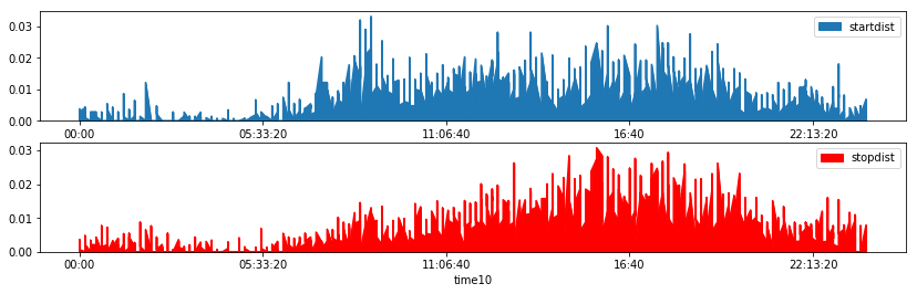
df = full
import matplotlib.pyplot as plt
fig, ax = plt.subplots(2, 1, figsize=(14,6))
df[df["station_id"] == 2].plot(x="time10", y="startdist", figsize=(14,4), kind="area", ax=ax[0])
df[df["station_id"] == 2].plot(x="time10", y="stopdist", figsize=(14,4),
                               kind="area", ax=ax[1], color="r");
Let’s build the features.
features = df.pivot_table(index=["station_id", "station_name", "weekday"],
                          columns="time10", values=["startdist", "stopdist"]).reset_index()

features.head()
| station_id | station_name | weekday | startdist | ... | stopdist | ||||||||||||||||
|---|---|---|---|---|---|---|---|---|---|---|---|---|---|---|---|---|---|---|---|---|---|
| time10 | 00:00:00 | 00:10:00 | 00:20:00 | 00:30:00 | 00:40:00 | 00:50:00 | 01:00:00 | ... | 22:20:00 | 22:30:00 | 22:40:00 | 22:50:00 | 23:00:00 | 23:10:00 | 23:20:00 | 23:30:00 | 23:40:00 | 23:50:00 | |||
| 0 | 2.0 | Michigan Ave & Balbo Ave | 0.0 | 0.003756 | 0.000939 | 0.002817 | 0.000000 | 0.000000 | 0.003756 | 0.000000 | ... | 0.004381 | 0.002191 | 0.004381 | 0.002191 | 0.004381 | 0.004381 | 0.005476 | 0.002191 | 0.000000 | 0.005476 |
| 1 | 2.0 | Michigan Ave & Balbo Ave | 1.0 | 0.000000 | 0.000000 | 0.001106 | 0.001106 | 0.001106 | 0.002212 | 0.000000 | ... | 0.009371 | 0.012048 | 0.006693 | 0.004016 | 0.005355 | 0.006693 | 0.002677 | 0.000000 | 0.000000 | 0.000000 |
| 2 | 2.0 | Michigan Ave & Balbo Ave | 2.0 | 0.001357 | 0.002714 | 0.000000 | 0.001357 | 0.000000 | 0.005427 | 0.000000 | ... | 0.002907 | 0.002907 | 0.015988 | 0.005814 | 0.001453 | 0.001453 | 0.011628 | 0.000000 | 0.000000 | 0.007267 |
| 3 | 2.0 | Michigan Ave & Balbo Ave | 3.0 | 0.000000 | 0.004144 | 0.000000 | 0.000000 | 0.002762 | 0.004144 | 0.000000 | ... | 0.009274 | 0.003091 | 0.003091 | 0.007728 | 0.001546 | 0.003091 | 0.009274 | 0.001546 | 0.007728 | 0.001546 |
| 4 | 2.0 | Michigan Ave & Balbo Ave | 4.0 | 0.000000 | 0.000000 | 0.000000 | 0.002846 | 0.000000 | 0.000000 | 0.000949 | ... | 0.008214 | 0.001027 | 0.006160 | 0.004107 | 0.015400 | 0.006160 | 0.002053 | 0.006160 | 0.007187 | 0.000000 |
5 rows × 291 columns
names = features.columns[3:]
len(names)
288
from sklearn.cluster import KMeans
clus = KMeans(8)
clus.fit(features[names])
KMeans(algorithm='auto', copy_x=True, init='k-means++', max_iter=300,
    n_clusters=8, n_init=10, n_jobs=1, precompute_distances='auto',
    random_state=None, tol=0.0001, verbose=0)
pred = clus.predict(features[names])
set(pred)
{0, 1, 2, 3, 4, 5, 6, 7}
features["cluster"] = pred
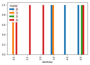
Let’s see what it means accross day. We need to look whether or not a cluster is related to day of the working week or the week end.
features[["cluster", "weekday", "station_id"]].groupby(["cluster", "weekday"]).count()
c:python370_x64libsite-packagespandascoregeneric.py:3111: PerformanceWarning: dropping on a non-lexsorted multi-index without a level parameter may impact performance.
  obj = obj._drop_axis(labels, axis, level=level, errors=errors)
| station_id | ||
|---|---|---|
| time10 | ||
| cluster | weekday | |
| 0 | 3.0 | 1 |
| 4.0 | 1 | |
| 6.0 | 1 | |
| 1 | 0.0 | 146 |
| 1.0 | 110 | |
| 2.0 | 106 | |
| 3.0 | 119 | |
| 4.0 | 143 | |
| 5.0 | 553 | |
| 6.0 | 547 | |
| 2 | 0.0 | 137 |
| 1.0 | 141 | |
| 2.0 | 150 | |
| 3.0 | 147 | |
| 4.0 | 149 | |
| 5.0 | 8 | |
| 6.0 | 12 | |
| 3 | 0.0 | 1 |
| 3.0 | 1 | |
| 4 | 2.0 | 1 |
| 3.0 | 1 | |
| 6.0 | 1 | |
| 5 | 6.0 | 1 |
| 6 | 0.0 | 1 |
| 1.0 | 1 | |
| 2.0 | 1 | |
| 6.0 | 1 | |
| 7 | 0.0 | 291 |
| 1.0 | 326 | |
| 2.0 | 322 | |
| 3.0 | 308 | |
| 4.0 | 287 | |
| 5.0 | 19 | |
| 6.0 | 17 |
nb = features[["cluster", "weekday", "station_id"]].groupby(["cluster", "weekday"]).count()
nb = nb.reset_index()
nb[nb.cluster.isin([0, 3, 5, 6])].pivot("weekday","cluster", "station_id").plot(kind="bar");
c:python370_x64libsite-packagespandascoregeneric.py:3111: PerformanceWarning: dropping on a non-lexsorted multi-index without a level parameter may impact performance.
  obj = obj._drop_axis(labels, axis, level=level, errors=errors)
Let’s draw the clusters.
centers = clus.cluster_centers_.T
import matplotlib.pyplot as plt
fig, ax = plt.subplots(centers.shape[1], 2, figsize=(10,10))
nbf = centers.shape[0] // 2
x = list(range(0,nbf))
col = 0
dec = 0
colors = ["red", "yellow", "gray", "green", "brown", "orange", "blue"]
for i in range(centers.shape[1]):
    if 2*i == centers.shape[1]:
        col += 1
        dec += centers.shape[1]
    color = colors[i%len(colors)]
    ax[2*i-dec, col].bar (x, centers[:nbf,i], width=1.0, color=color)
    ax[2*i-dec, col].set_ylabel("cluster %d - start" % i, color=color)
    ax[2*i+1-dec, col].bar (x, centers[nbf:,i], width=1.0, color=color)
    ax[2*i+1-dec, col].set_ylabel("cluster %d - stop" % i, color=color)
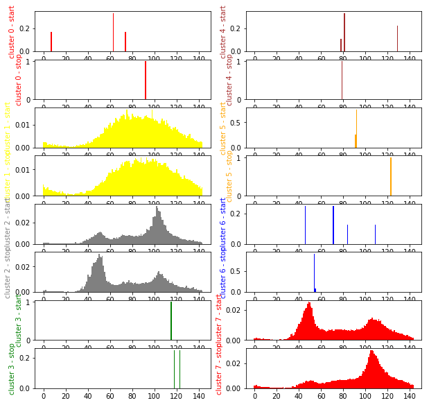
Four patterns emerge. Small clusters are annoying but let’s show them on a map. The widest one is the one for the week-end.
Graph#
We first need to get 7 clusters for each stations, one per day.
piv = features.pivot_table(index=["station_id","station_name"],
                           columns="weekday", values="cluster")
piv.head()
c:python370_x64libsite-packagespandascoregeneric.py:3111: PerformanceWarning: dropping on a non-lexsorted multi-index without a level parameter may impact performance.
  obj = obj._drop_axis(labels, axis, level=level, errors=errors)
| time10 | ||||||||
|---|---|---|---|---|---|---|---|---|
| weekday | 0.0 | 1.0 | 2.0 | 3.0 | 4.0 | 5.0 | 6.0 | |
| station_id | station_name | |||||||
| 2.0 | Michigan Ave & Balbo Ave | 1.0 | 7.0 | 1.0 | 1.0 | 1.0 | 1.0 | 1.0 |
| 3.0 | Shedd Aquarium | 1.0 | 1.0 | 1.0 | 1.0 | 1.0 | 1.0 | 1.0 |
| 4.0 | Burnham Harbor | 1.0 | 1.0 | 1.0 | 1.0 | 1.0 | 1.0 | 1.0 |
| 5.0 | State St & Harrison St | 7.0 | 7.0 | 7.0 | 7.0 | 7.0 | 1.0 | 1.0 |
| 6.0 | Dusable Harbor | 1.0 | 1.0 | 1.0 | 1.0 | 1.0 | 1.0 | 1.0 |
piv["distincts"] = piv.apply(lambda row: len(set(row[i] for i in range(0,7))), axis=1)
Let’s see which station is classified in more than 4 clusters. NaN means no bikes stopped at this stations. They are mostly unused stations.
piv[piv.distincts >= 4]
| time10 | distincts | ||||||||
|---|---|---|---|---|---|---|---|---|---|
| weekday | 0.0 | 1.0 | 2.0 | 3.0 | 4.0 | 5.0 | 6.0 | ||
| station_id | station_name | ||||||||
| 391.0 | Halsted St & 69th St | 3.0 | 7.0 | 1.0 | 7.0 | 1.0 | 1.0 | 2.0 | 4 |
| 440.0 | Lawndale Ave & 23rd St | 7.0 | 7.0 | 1.0 | 7.0 | 2.0 | 1.0 | 0.0 | 4 |
| 557.0 | Damen Ave & Garfield Blvd | NaN | 2.0 | 1.0 | NaN | 2.0 | NaN | NaN | 6 |
| 558.0 | Ashland Ave & Garfield Blvd | NaN | 1.0 | 1.0 | 1.0 | 1.0 | 2.0 | NaN | 4 |
| 561.0 | Damen Ave & 61st St | 2.0 | 7.0 | 2.0 | 7.0 | NaN | 1.0 | 1.0 | 4 |
| 562.0 | Racine Ave & 61st St | NaN | NaN | NaN | NaN | 7.0 | NaN | NaN | 7 |
| 564.0 | Racine Ave & 65th St | 1.0 | 1.0 | NaN | NaN | 7.0 | 1.0 | 7.0 | 4 |
| 565.0 | Ashland Ave & 66th St | 1.0 | 1.0 | NaN | 1.0 | 0.0 | NaN | 5.0 | 5 |
| 567.0 | May St & 69th St | 6.0 | 6.0 | 2.0 | 2.0 | 1.0 | 1.0 | NaN | 4 |
| 568.0 | Normal Ave & 72nd St | 1.0 | 1.0 | 7.0 | NaN | 7.0 | 1.0 | 4.0 | 4 |
| 569.0 | Woodlawn Ave & 75th St | 1.0 | NaN | 7.0 | 1.0 | 1.0 | NaN | 1.0 | 4 |
| 576.0 | Greenwood Ave & 79th St | 7.0 | 1.0 | 1.0 | NaN | 2.0 | 1.0 | 1.0 | 4 |
| 581.0 | Commercial Ave & 83rd St | 1.0 | NaN | 7.0 | NaN | NaN | 1.0 | 1.0 | 5 |
| 582.0 | Phillips Ave & 82nd St | NaN | NaN | 1.0 | 1.0 | NaN | 1.0 | 7.0 | 5 |
| 586.0 | MLK Jr Dr & 83rd St | 1.0 | 2.0 | 6.0 | 7.0 | 7.0 | 7.0 | 2.0 | 4 |
| 587.0 | Wabash Ave & 83rd St | NaN | NaN | 1.0 | NaN | 1.0 | 2.0 | 7.0 | 6 |
| 588.0 | South Chicago Ave & 83rd St | NaN | 2.0 | 7.0 | 3.0 | 1.0 | 2.0 | 7.0 | 5 |
| 593.0 | Halsted St & 59th St | NaN | 7.0 | 4.0 | 4.0 | NaN | 1.0 | 1.0 | 5 |
pivn = piv.reset_index()
pivn.columns = [' '.join(str(_).replace(".0", "") for _ in col).strip() for col in pivn.columns.values]
pivn.head()
| station_id | station_name | 0 | 1 | 2 | 3 | 4 | 5 | 6 | distincts | |
|---|---|---|---|---|---|---|---|---|---|---|
| 0 | 2.0 | Michigan Ave & Balbo Ave | 1.0 | 7.0 | 1.0 | 1.0 | 1.0 | 1.0 | 1.0 | 2 |
| 1 | 3.0 | Shedd Aquarium | 1.0 | 1.0 | 1.0 | 1.0 | 1.0 | 1.0 | 1.0 | 1 |
| 2 | 4.0 | Burnham Harbor | 1.0 | 1.0 | 1.0 | 1.0 | 1.0 | 1.0 | 1.0 | 1 |
| 3 | 5.0 | State St & Harrison St | 7.0 | 7.0 | 7.0 | 7.0 | 7.0 | 1.0 | 1.0 | 2 |
| 4 | 6.0 | Dusable Harbor | 1.0 | 1.0 | 1.0 | 1.0 | 1.0 | 1.0 | 1.0 | 1 |
Let’s draw a map on a week day.
data = stations.merge(pivn, left_on=["id", "name"],
                      right_on=["station_id", "station_name"], suffixes=('_s', '_c'))
data.sort_values("id").head()
| id | name | latitude | longitude | dpcapacity | online_date | station_id | station_name | 0 | 1 | 2 | 3 | 4 | 5 | 6 | distincts | |
|---|---|---|---|---|---|---|---|---|---|---|---|---|---|---|---|---|
| 357 | 2 | Michigan Ave & Balbo Ave | 41.872638 | -87.623979 | 35 | 5/8/2015 | 2.0 | Michigan Ave & Balbo Ave | 1.0 | 7.0 | 1.0 | 1.0 | 1.0 | 1.0 | 1.0 | 2 |
| 456 | 3 | Shedd Aquarium | 41.867226 | -87.615355 | 31 | 4/24/2015 | 3.0 | Shedd Aquarium | 1.0 | 1.0 | 1.0 | 1.0 | 1.0 | 1.0 | 1.0 | 1 |
| 53 | 4 | Burnham Harbor | 41.856268 | -87.613348 | 23 | 5/16/2015 | 4.0 | Burnham Harbor | 1.0 | 1.0 | 1.0 | 1.0 | 1.0 | 1.0 | 1.0 | 1 |
| 497 | 5 | State St & Harrison St | 41.874053 | -87.627716 | 23 | 6/18/2013 | 5.0 | State St & Harrison St | 7.0 | 7.0 | 7.0 | 7.0 | 7.0 | 1.0 | 1.0 | 2 |
| 188 | 6 | Dusable Harbor | 41.885042 | -87.612795 | 31 | 4/24/2015 | 6.0 | Dusable Harbor | 1.0 | 1.0 | 1.0 | 1.0 | 1.0 | 1.0 | 1.0 | 1 |
from ensae_projects.datainc.data_bikes import folium_html_stations_map

colors = ["red", "yellow", "gray", "green", "brown", "orange", "blue", "black"]
for i, c in enumerate(colors):
    print("Cluster {0} is {1}".format(i, c))
xy = []
for els in data.apply(lambda row: (row["latitude"], row["longitude"], row["1"], row["name"]), axis=1):
    try:
        cl = int(els[2])
    except:
        # NaN
        continue
    name = "%s c%d" % (els[3], cl)
    color = colors[cl]
    xy.append( ( (els[0], els[1]), (name, color)))
folium_html_stations_map(xy, width="80%")
Cluster 0 is red
Cluster 1 is yellow
Cluster 2 is gray
Cluster 3 is green
Cluster 4 is brown
Cluster 5 is orange
Cluster 6 is blue
Cluster 7 is black
Look at the colors close the parks. We notice than people got to the park after work. Let’s see during the week-end.
xy = []
for els in data.apply(lambda row: (row["latitude"], row["longitude"], row["5"], row["name"]), axis=1):
    try:
        cl = int(els[2])
    except:
        # NaN
        continue
    name = "%s c%d" % (els[3], cl)
    color = colors[cl]
    xy.append( ( (els[0], els[1]), (name, color)))
folium_html_stations_map(xy, width="80%")