City Bike Views

Links: notebook, html, PDF, python, slides, GitHub

Based on the data available at Divvy Data, some ways to look at the data.

from jyquickhelper import add_notebook_menu
add_notebook_menu()

%matplotlib inline

The data

Divvy Data publishes a sample of the data.

from pyensae.datasource import download_data
file = download_data("Divvy_Trips_2016_Q3Q4.zip", url="https://s3.amazonaws.com/divvy-data/tripdata/")

import pandas
stations = pandas.read_csv("Divvy_Stations_2016_Q3.csv")
bikes = pandas.concat([pandas.read_csv("Divvy_Trips_2016_Q3.csv"),
                       pandas.read_csv("Divvy_Trips_2016_Q4.csv")])

bikes.head()

	trip_id	starttime	stoptime	bikeid	tripduration	from_station_id	from_station_name	to_station_id	to_station_name	usertype	gender	birthyear
0	12150160	9/30/2016 23:59:58	10/1/2016 00:04:03	4959	245	69	Damen Ave & Pierce Ave	17	Wood St & Division St	Subscriber	Male	1988.0
1	12150159	9/30/2016 23:59:58	10/1/2016 00:04:09	2589	251	383	Ashland Ave & Harrison St	320	Loomis St & Lexington St	Subscriber	Female	1990.0
2	12150158	9/30/2016 23:59:51	10/1/2016 00:24:51	3656	1500	302	Sheffield Ave & Wrightwood Ave	334	Lake Shore Dr & Belmont Ave	Customer	NaN	NaN
3	12150157	9/30/2016 23:59:51	10/1/2016 00:03:56	3570	245	475	Washtenaw Ave & Lawrence Ave	471	Francisco Ave & Foster Ave	Subscriber	Female	1988.0
4	12150156	9/30/2016 23:59:32	10/1/2016 00:26:50	3158	1638	302	Sheffield Ave & Wrightwood Ave	492	Leavitt St & Addison St	Customer	NaN	NaN

About age

from datetime import datetime, time
df = bikes
df["dtstart"] = pandas.to_datetime(df.starttime, infer_datetime_format=True)
df["dtstop"] = pandas.to_datetime(df.stoptime, infer_datetime_format=True)
df["stopday"] = df.dtstop.apply(lambda r: datetime(r.year, r.month, r.day))
df["stoptime"] = df.dtstop.apply(lambda r: time(r.hour, r.minute, 0))
df["stoptime10"] = df.dtstop.apply(lambda r: time(r.hour, (r.minute // 10)*10, 0))  # every 10 minutes
df['stopweekday'] = df['dtstop'].dt.dayofweek

df['duration'] = df["dtstop"] -  df["dtstart"]
df["age"] = - df["birthyear"] + 2016
df['duration_sec'] = df['duration'].apply(lambda x: x.total_seconds())

df["stoptime_sec"] = df.dtstop.apply(lambda r: r.hour * 60 + r.minute)

df.describe().T

	count	mean	std	min	25%	50%	75%	max
trip_id	2.12564e+06	1.16993e+07	731388	1.04267e+07	1.10663e+07	1.17015e+07	1.23313e+07	1.29792e+07
bikeid	2.12564e+06	3251.98	1730.44	1	1755	3446	4802	5920
tripduration	2.12564e+06	1008.55	1816.1	60	416	716	1195	86365
from_station_id	2.12564e+06	179.916	130.524	2	75	157	268	620
to_station_id	2.12564e+06	180.352	130.488	2	75	157	272	620
birthyear	1.59034e+06	1980.79	10.754	1899	1975	1984	1989	2000
stopweekday	2.12564e+06	2.95275	2.02016	0	1	3	5	6
duration	2125643	0 days 00:16:48.183487	0 days 00:30:15.597468	0 days 00:00:59	0 days 00:06:56	0 days 00:11:56	0 days 00:19:55	0 days 23:59:24
age	1.59034e+06	35.2129	10.754	16	27	32	41	117
duration_sec	2.12564e+06	1008.18	1815.6	59	416	716	1195	86364
stoptime_sec	2.12564e+06	869.324	284.732	0	652	919	1080	1439

df.shape

(2125643, 21)

We take a random sample.

import random
ens = pandas.Series([random.randint(0,99) for i in range(df.shape[0])])
sample = df[ens==0]

c:python370_x64libsite-packagesipykernel_launcher.py:3: UserWarning: Boolean Series key will be reindexed to match DataFrame index.
  This is separate from the ipykernel package so we can avoid doing imports until

sample.shape
sample = sample[(sample.age < 100) & (sample.duration_sec < 3600)]

import numpy as np
import pandas as pd
import seaborn as sns
sns.set(style="white")
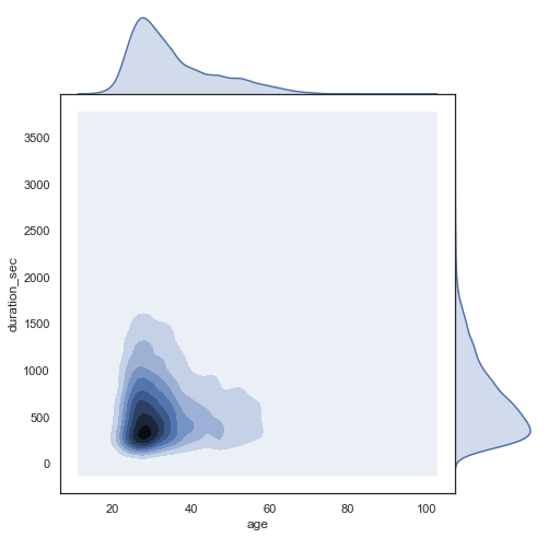
g = sns.jointplot(sample.age, sample.duration_sec, kind="kde", size=7, space=0)

c:python370_x64libsite-packagesseabornaxisgrid.py:2262: UserWarning: The size paramter has been renamed to height; please update your code.
  warnings.warn(msg, UserWarning)
c:python370_x64libsite-packagesscipystatsstats.py:1713: FutureWarning: Using a non-tuple sequence for multidimensional indexing is deprecated; use arr[tuple(seq)] instead of arr[seq]. In the future this will be interpreted as an array index, arr[np.array(seq)], which will result either in an error or a different result.
  return np.add.reduce(sorted[indexer] * weights, axis=axis) / sumval

import numpy as np
import pandas as pd
import seaborn as sns
sns.set(style="white")
g = sns.jointplot(sample.age, sample.stoptime_sec, kind="kde", size=7, space=0)

c:python370_x64libsite-packagesseabornaxisgrid.py:2262: UserWarning: The size paramter has been renamed to height; please update your code.
  warnings.warn(msg, UserWarning)
c:python370_x64libsite-packagesscipystatsstats.py:1713: FutureWarning: Using a non-tuple sequence for multidimensional indexing is deprecated; use arr[tuple(seq)] instead of arr[seq]. In the future this will be interpreted as an array index, arr[np.array(seq)], which will result either in an error or a different result.
  return np.add.reduce(sorted[indexer] * weights, axis=axis) / sumval

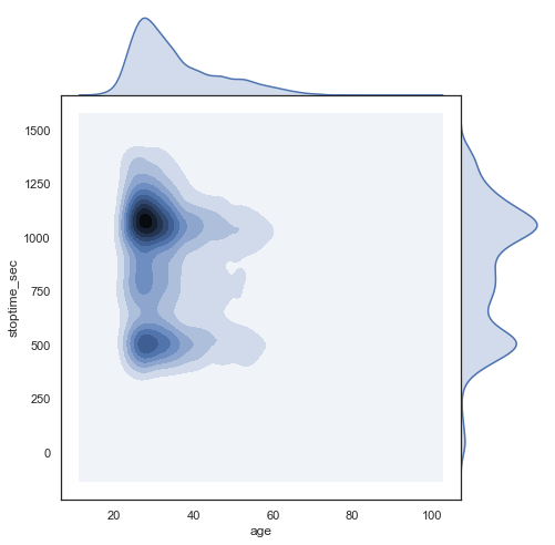
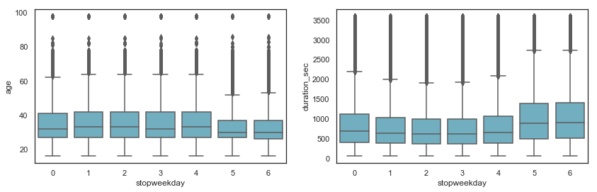
The duration seems correlated to the age. Let’s see. Younger people during the weekend are more active and bike longer.

import matplotlib.pyplot as plt
fig, ax = plt.subplots(1,2, figsize=(14,4))
sns.boxplot(x="stopweekday", y="age", data=df[df.age < 100], color="c", ax=ax[0])
sns.boxplot(x="stopweekday", y="duration_sec", data=df[df.duration_sec < 3600], color="c", ax=ax[1]);

However, linear correlations are not so great.

df.corr()

	trip_id	bikeid	tripduration	from_station_id	to_station_id	birthyear	stopweekday	age	duration_sec	stoptime_sec
trip_id	1.000000	-0.025039	-0.071566	0.008129	0.005505	-0.035032	-0.067585	0.035032	-0.071514	-0.063709
bikeid	-0.025039	1.000000	0.001088	0.009959	0.009538	-0.010901	0.000779	0.010901	0.001090	-0.007245
tripduration	-0.071566	0.001088	1.000000	-0.008972	-0.004730	-0.009788	0.069885	0.009788	0.999969	0.034435
from_station_id	0.008129	0.009959	-0.008972	1.000000	0.386314	0.019982	0.019426	-0.019982	-0.008970	-0.016486
to_station_id	0.005505	0.009538	-0.004730	0.386314	1.000000	0.021198	0.011177	-0.021198	-0.004734	0.061833
birthyear	-0.035032	-0.010901	-0.009788	0.019982	0.021198	1.000000	0.057081	-1.000000	-0.009808	0.085929
stopweekday	-0.067585	0.000779	0.069885	0.019426	0.011177	0.057081	1.000000	-0.057081	0.069848	0.017866
age	0.035032	0.010901	0.009788	-0.019982	-0.021198	-1.000000	-0.057081	1.000000	0.009808	-0.085929
duration_sec	-0.071514	0.001090	0.999969	-0.008970	-0.004734	-0.009808	0.069848	0.009808	1.000000	0.034514
stoptime_sec	-0.063709	-0.007245	0.034435	-0.016486	0.061833	0.085929	0.017866	-0.085929	0.034514	1.000000

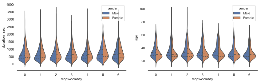
fig, ax = plt.subplots(1,2, figsize=(14,4))
sns.violinplot(x="stopweekday", y="duration_sec", hue="gender", data=sample, split=True, inner="quart", ax=ax[0])
sns.violinplot(x="stopweekday", y="age", hue="gender", data=sample, split=True, inner="quart", ax=ax[1])
sns.despine(left=True);

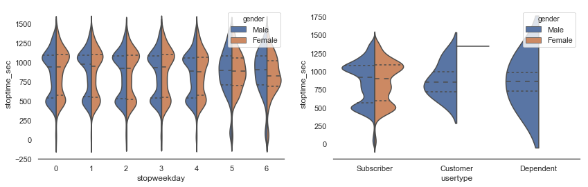
fig, ax = plt.subplots(1,2, figsize=(14,4))
sns.violinplot(x="stopweekday", y="stoptime_sec", hue="gender", data=sample, split=True, inner="quart", ax=ax[0])
sns.violinplot(x="usertype", y="stoptime_sec", hue="gender", data=sample, split=True, inner="quart", ax=ax[1])
sns.despine(left=True);

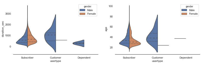
fig, ax = plt.subplots(1,2, figsize=(14,4))
sns.violinplot(x="usertype", y="duration_sec", hue="gender", data=sample, split=True, inner="quart", ax=ax[0])
sns.violinplot(x="usertype", y="age", hue="gender", data=sample, split=True, inner="quart", ax=ax[1])
sns.despine(left=True);

Non-linear correlations

We apply the following Corrélations non linéaires.

sample2 = sample.copy()
sample2["age_inv"] = sample2.age ** -1
sample2["gender_num"] = sample2.gender.apply(lambda x: (1 if x == "Male" else 0))
sample2["usertype_num"] = sample2.usertype.apply(lambda x: (1 if x == "Subscriber" else 0))
sample2.corr()

	trip_id	bikeid	tripduration	from_station_id	to_station_id	birthyear	stopweekday	age	duration_sec	stoptime_sec	age_inv	gender_num	usertype_num
trip_id	1.000000	-0.020790	-0.090476	-0.000107	-0.013945	-0.032304	-0.044524	0.032304	-0.089994	-0.050106	-0.027614	0.058240	0.014886
bikeid	-0.020790	1.000000	0.011953	0.009183	0.013776	-0.011606	-0.001548	0.011606	0.011944	-0.004755	-0.009776	0.031241	-0.000271
tripduration	-0.090476	0.011953	1.000000	0.044958	0.050456	-0.005926	0.063156	0.005926	0.999999	0.073529	-0.016003	-0.108492	-0.008061
from_station_id	-0.000107	0.009183	0.044958	1.000000	0.381516	0.021112	0.051470	-0.021112	0.044957	-0.010079	0.029148	-0.027132	0.019338
to_station_id	-0.013945	0.013776	0.050456	0.381516	1.000000	0.027436	0.049334	-0.027436	0.050440	0.089843	0.033983	-0.031992	0.014013
birthyear	-0.032304	-0.011606	-0.005926	0.021112	0.027436	1.000000	0.047890	-1.000000	-0.005937	0.090793	0.951178	-0.080894	0.008748
stopweekday	-0.044524	-0.001548	0.063156	0.051470	0.049334	0.047890	1.000000	-0.047890	0.063146	-0.005645	0.052167	-0.043754	-0.009274
age	0.032304	0.011606	0.005926	-0.021112	-0.027436	-1.000000	-0.047890	1.000000	0.005937	-0.090793	-0.951178	0.080894	-0.008748
duration_sec	-0.089994	0.011944	0.999999	0.044957	0.050440	-0.005937	0.063146	0.005937	1.000000	0.073511	-0.016010	-0.108476	-0.008063
stoptime_sec	-0.050106	-0.004755	0.073529	-0.010079	0.089843	0.090793	-0.005645	-0.090793	0.073511	1.000000	0.091370	-0.003124	-0.005995
age_inv	-0.027614	-0.009776	-0.016003	0.029148	0.033983	0.951178	0.052167	-0.951178	-0.016010	0.091370	1.000000	-0.088716	0.009361
gender_num	0.058240	0.031241	-0.108492	-0.027132	-0.031992	-0.080894	-0.043754	0.080894	-0.108476	-0.003124	-0.088716	1.000000	-0.009875
usertype_num	0.014886	-0.000271	-0.008061	0.019338	0.014013	0.008748	-0.009274	-0.008748	-0.008063	-0.005995	0.009361	-0.009875	1.000000

from sklearn.model_selection import train_test_split
from sklearn.preprocessing import scale
import numpy

def correlation_cross_val(df, model, draws=5, **params):
    cor = df.corr()
    df = scale(df[cor.columns])
    for i in range(cor.shape[0]):
        xi = df[:, i:i+1]
        for j in range(cor.shape[1]):
            xj = df[:, j]
            mem = []
            for k in range(0, draws):
                xi_train, xi_test, xj_train, xj_test = train_test_split(xi, xj, train_size=0.5)
                mod = model(**params)
                mod.fit(xi_train, xj_train)
                v = mod.predict(xi_test)
                c = (1 - numpy.var(v - xj_test))
                mem.append(max(c, 0) **0.5)
            cor.iloc[i,j] = sum(mem) / len(mem)
    return cor

from sklearn.tree import DecisionTreeRegressor
cor = correlation_cross_val(sample2, DecisionTreeRegressor, draws=20)
cor

c:python370_x64libsite-packagessklearnmodel_selection_split.py:2026: FutureWarning: From version 0.21, test_size will always complement train_size unless both are specified.
  FutureWarning)

	trip_id	bikeid	tripduration	from_station_id	to_station_id	birthyear	stopweekday	age	duration_sec	stoptime_sec	age_inv	gender_num	usertype_num
trip_id	1.000000	0.000000	0.000000	0.000000	0.000000	0.000000	0.990057	0.000000	0.000000	0.878676	0.000000	0.000000	0.015071
bikeid	0.000000	1.000000	0.000000	0.000000	0.000000	0.000000	0.000000	0.000000	0.000000	0.000000	0.000000	0.000000	0.017745
tripduration	0.000000	0.000000	0.999990	0.000000	0.000000	0.000000	0.000000	0.000000	0.999990	0.000000	0.000000	0.000000	0.099688
from_station_id	0.000000	0.000000	0.054325	0.999999	0.536015	0.008031	0.000000	0.006133	0.044061	0.012246	0.028895	0.000000	0.172352
to_station_id	0.000000	0.000000	0.109784	0.532589	0.999999	0.026304	0.000000	0.024202	0.105040	0.248720	0.019269	0.000000	0.153788
birthyear	0.011917	0.005125	0.058987	0.026033	0.034188	0.999965	0.006681	0.999942	0.053868	0.055993	0.999996	0.068499	0.209815
stopweekday	0.042561	0.020920	0.079774	0.065344	0.045880	0.085778	1.000000	0.055188	0.074982	0.033219	0.095588	0.054960	0.291366
age	0.011934	0.006577	0.051631	0.019733	0.028614	0.999909	0.017197	0.999943	0.063061	0.052308	0.999997	0.055599	0.332540
duration_sec	0.000000	0.000000	0.999991	0.000000	0.000000	0.000000	0.000000	0.000000	0.999992	0.000000	0.000000	0.000000	0.026094
stoptime_sec	0.000000	0.000000	0.000000	0.000000	0.000000	0.000000	0.000000	0.000000	0.000000	1.000000	0.000000	0.000000	0.114911
age_inv	0.017233	0.009412	0.042053	0.028141	0.010642	0.999918	0.024621	0.999912	0.022328	0.051536	0.999997	0.070596	0.275990
gender_num	0.049358	0.032177	0.073034	0.038476	0.065741	0.080659	0.039153	0.062295	0.079421	0.052172	0.085579	1.000000	0.245688
usertype_num	0.032215	0.041777	0.063852	0.039527	0.032406	0.038315	0.037363	0.055648	0.059596	0.037164	0.039390	0.035496	1.000000

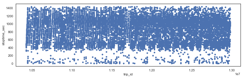
from_station_id and start_station_id seem related. Which means there is frequent trip. Funny, the trip id can explain the stopping time… It should be removed from any dataset.

sample2.plot(x="trip_id", y="stoptime_sec", kind="scatter", figsize=(14,4));