2A.ML101.4: Supervised Learning: Regression of Housing Data

Links: notebook, html, PDF, python, slides, GitHub

Here we’ll do a short example of a regression problem: learning a continuous value from a set of features.

We’ll use the simple Boston house prices set, available in scikit-learn. This records measurements of 13 attributes of housing markets around Boston, as well as the median price. The question is: can you predict the price of a new market given its attributes?

Source: Course on machine learning with scikit-learn by Gaël Varoquaux

from sklearn.datasets import load_boston
data = load_boston()
print(data.data.shape)
print(data.target.shape)

(506, 13)
(506,)

We can see that there are just over 500 data points.

The DESCR variable has a long description of the dataset:

print(data.DESCR)

Boston House Prices dataset
===========================
Notes
------
Data Set Characteristics:
    :Number of Instances: 506
    :Number of Attributes: 13 numeric/categorical predictive
    :Median Value (attribute 14) is usually the target
    :Attribute Information (in order):
        - CRIM     per capita crime rate by town
        - ZN       proportion of residential land zoned for lots over 25,000 sq.ft.
        - INDUS    proportion of non-retail business acres per town
        - CHAS     Charles River dummy variable (= 1 if tract bounds river; 0 otherwise)
        - NOX      nitric oxides concentration (parts per 10 million)
        - RM       average number of rooms per dwelling
        - AGE      proportion of owner-occupied units built prior to 1940
        - DIS      weighted distances to five Boston employment centres
        - RAD      index of accessibility to radial highways
        - TAX      full-value property-tax rate per $10,000
        - PTRATIO  pupil-teacher ratio by town
        - B        1000(Bk - 0.63)^2 where Bk is the proportion of blacks by town
        - LSTAT    % lower status of the population
        - MEDV     Median value of owner-occupied homes in $1000's
    :Missing Attribute Values: None
    :Creator: Harrison, D. and Rubinfeld, D.L.
This is a copy of UCI ML housing dataset.
http://archive.ics.uci.edu/ml/datasets/Housing

This dataset was taken from the StatLib library which is maintained at Carnegie Mellon University.
The Boston house-price data of Harrison, D. and Rubinfeld, D.L. 'Hedonic
prices and the demand for clean air', J. Environ. Economics & Management,
vol.5, 81-102, 1978.   Used in Belsley, Kuh & Welsch, 'Regression diagnostics
...', Wiley, 1980.   N.B. Various transformations are used in the table on
pages 244-261 of the latter.
The Boston house-price data has been used in many machine learning papers that address regression
problems.
References
   - Belsley, Kuh & Welsch, 'Regression diagnostics: Identifying Influential Data and Sources of Collinearity', Wiley, 1980. 244-261.
   - Quinlan,R. (1993). Combining Instance-Based and Model-Based Learning. In Proceedings on the Tenth International Conference of Machine Learning, 236-243, University of Massachusetts, Amherst. Morgan Kaufmann.
   - many more! (see http://archive.ics.uci.edu/ml/datasets/Housing)

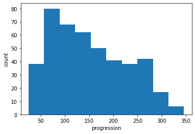
It often helps to quickly visualize pieces of the data using histograms, scatter plots, or other plot types. Here we’ll load pylab and show a histogram of the target values: the median price in each neighborhood.

%matplotlib inline
import matplotlib.pyplot as plt
import numpy as np

plt.hist(data.target)
plt.xlabel('price ($1000s)')
plt.ylabel('count');

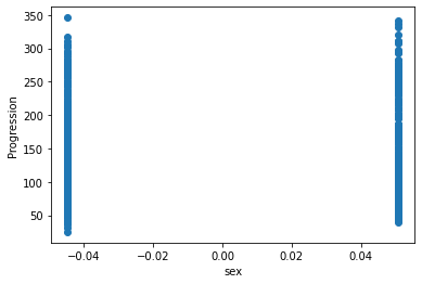
Let’s have a quick look to see if some features are more relevant than others for our problem

for index, feature_name in enumerate(data.feature_names):
    plt.figure()
    plt.scatter(data.data[:, index], data.target)
    plt.ylabel('Price')
    plt.xlabel(feature_name)

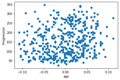
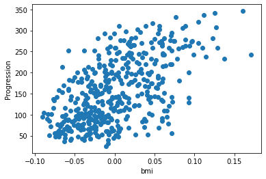
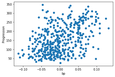
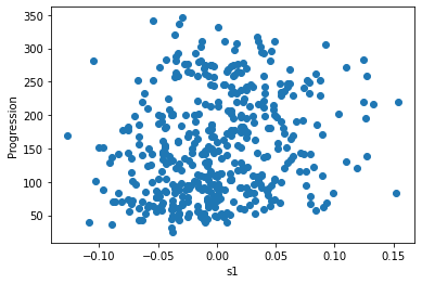
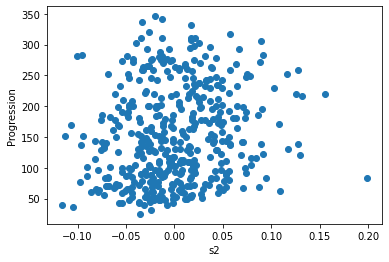
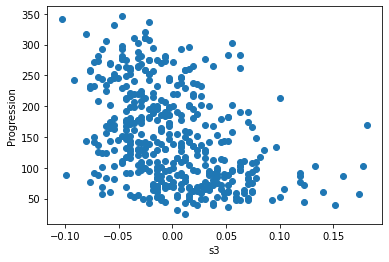
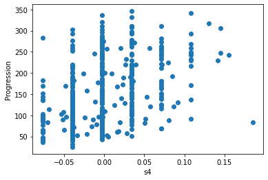
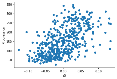
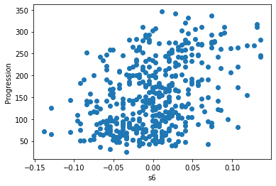
This is a manual version of a technique called feature selection.

Sometimes, in Machine Learning it is useful to use feature selection to decide which features are most useful for a particular problem. Automated methods exist which quantify this sort of exercise of choosing the most informative features.

Predicting Home Prices: a Simple Linear Regression

Now we’ll use scikit-learn to perform a simple linear regression on the housing data. There are many possibilities of regressors to use. A particularly simple one is LinearRegression: this is basically a wrapper around an ordinary least squares calculation.

We’ll set it up like this:

from sklearn.model_selection import train_test_split

X_train, X_test, y_train, y_test = train_test_split(data.data, data.target)

from sklearn.linear_model import LinearRegression

clf = LinearRegression()
clf.fit(X_train, y_train)

LinearRegression(copy_X=True, fit_intercept=True, n_jobs=1, normalize=False)

predicted = clf.predict(X_test)
expected = y_test

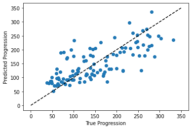
plt.scatter(expected, predicted)
plt.plot([0, 50], [0, 50], '--k')
plt.axis('tight')
plt.xlabel('True price ($1000s)')
plt.ylabel('Predicted price ($1000s)')
print("RMS:", np.sqrt(np.mean((predicted - expected) ** 2)))

RMS: 5.517282984386352

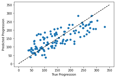
The prediction at least correlates with the true price, though there are clearly some biases. We could imagine evaluating the performance of the regressor by, say, computing the RMS residuals between the true and predicted price. There are some subtleties in this, however, which we’ll cover in a later section.

Exercise: Gradient Boosting Tree Regression

There are many other types of regressors available in scikit-learn: we’ll try a more powerful one here.

Use the GradientBoostingRegressor class to fit the housing data.

You can copy and paste some of the above code, replacing LinearRegression with GradientBoostingRegressor.

from sklearn.ensemble import GradientBoostingRegressor
# Instantiate the model, fit the results, and scatter in vs. out

c:python370_x64libsite-packagessklearnensembleweight_boosting.py:29: DeprecationWarning: numpy.core.umath_tests is an internal NumPy module and should not be imported. It will be removed in a future NumPy release.
  from numpy.core.umath_tests import inner1d

Solution:

from sklearn.ensemble import GradientBoostingRegressor

clf = GradientBoostingRegressor()
clf.fit(X_train, y_train)

predicted = clf.predict(X_test)
expected = y_test

plt.scatter(expected, predicted)
plt.plot([0, 50], [0, 50], '--k')
plt.axis('tight')
plt.xlabel('True price ($1000s)')
plt.ylabel('Predicted price ($1000s)')
print("RMS:", np.sqrt(np.mean((predicted - expected) ** 2)))

RMS: 3.309772461419991