2A.ML101.1: Introduction to data manipulation with scientific Python#
Links: notebook, html, python, slides, GitHub
In this section we’ll go through the basics of the scientific Python stack for data manipulation: using numpy and matplotlib.
Source: Course on machine learning with scikit-learn by Gaël Varoquaux
You can skip this section if you already know the scipy stack.
To learn the scientific Python ecosystem: http://scipy-lectures.org
# Start pylab inline mode, so figures will appear in the notebook
%matplotlib inline
Numpy Arrays#
Manipulating numpy arrays is an important part of doing machine
learning (or, really, any type of scientific computation) in Python.
This will likely be review for most: we’ll quickly go through some of
the most important features.
import numpy as np

# Generating a random array
X = np.random.random((3, 5))  # a 3 x 5 array

print(X)
[[0.93806505 0.88546824 0.72716304 0.04025777 0.89691774]
 [0.54692084 0.56108889 0.77577327 0.62409764 0.17180018]
 [0.96342087 0.60346547 0.16957905 0.58235256 0.22502235]]
# Accessing elements

# get a single element
print(X[0, 0])

# get a row
print(X[1])

# get a column
print(X[:, 1])
0.9380650481256236
[0.54692084 0.56108889 0.77577327 0.62409764 0.17180018]
[0.88546824 0.56108889 0.60346547]
# Transposing an array
print(X.T)
[[0.93806505 0.54692084 0.96342087]
 [0.88546824 0.56108889 0.60346547]
 [0.72716304 0.77577327 0.16957905]
 [0.04025777 0.62409764 0.58235256]
 [0.89691774 0.17180018 0.22502235]]
# Turning a row vector into a column vector
y = np.linspace(0, 12, 5)
print(y)
[ 0. 3. 6. 9. 12.]
# make into a column vector
print(y[:, np.newaxis])
[[ 0.]
 [ 3.]
 [ 6.]
 [ 9.]
 [12.]]
There is much, much more to know, but these few operations are fundamental to what we’ll do during this tutorial.
Scipy Sparse Matrices#
We won’t make very much use of these in this tutorial, but sparse matrices are very nice in some situations. For example, in some machine learning tasks, especially those associated with textual analysis, the data may be mostly zeros. Storing all these zeros is very inefficient. We can create and manipulate sparse matrices as follows:
from scipy import sparse

# Create a random array with a lot of zeros
X = np.random.random((10, 5))
print(X)
[[0.41799001 0.20034867 0.60892716 0.25861014 0.63509755]
 [0.65058502 0.0098216  0.13038958 0.03960645 0.55062935]
 [0.94271976 0.28736949 0.21038553 0.49161759 0.11113543]
 [0.80481651 0.09016237 0.40425573 0.56510904 0.53661611]
 [0.079217   0.15374011 0.76457524 0.1097451  0.91216209]
 [0.21447349 0.7089186  0.70915116 0.44892699 0.80017261]
 [0.67488076 0.02466962 0.67453018 0.00671606 0.21792525]
 [0.61421541 0.41031706 0.05108445 0.18081791 0.9790548 ]
 [0.91433767 0.15576258 0.07304524 0.53041295 0.46649357]
 [0.83730157 0.89792046 0.7531655  0.05661956 0.13875142]]
# set the majority of elements to zero
X[X < 0.7] = 0
print(X)
[[0.         0.         0.         0.         0.        ]
 [0.         0.         0.         0.         0.        ]
 [0.94271976 0.         0.         0.         0.        ]
 [0.80481651 0.         0.         0.         0.        ]
 [0.         0.         0.76457524 0.         0.91216209]
 [0.         0.7089186  0.70915116 0.         0.80017261]
 [0.         0.         0.         0.         0.        ]
 [0.         0.         0.         0.         0.9790548 ]
 [0.91433767 0.         0.         0.         0.        ]
 [0.83730157 0.89792046 0.7531655  0.         0.        ]]
# turn X into a csr (Compressed-Sparse-Row) matrix
X_csr = sparse.csr_matrix(X)
print(X_csr)
(2, 0)    0.9427197583439572
(3, 0)    0.8048165053861909
(4, 2)    0.7645752378228468
(4, 4)    0.9121620939410845
(5, 1)    0.708918601388826
(5, 2)    0.7091511593075851
(5, 4)    0.800172608559929
(7, 4)    0.9790548029613194
(8, 0)    0.9143376669464592
(9, 0)    0.837301565304061
(9, 1)    0.8979204572473508
(9, 2)    0.7531655008508734
# convert the sparse matrix to a dense array
print(X_csr.toarray())
[[0.         0.         0.         0.         0.        ]
 [0.         0.         0.         0.         0.        ]
 [0.94271976 0.         0.         0.         0.        ]
 [0.80481651 0.         0.         0.         0.        ]
 [0.         0.         0.76457524 0.         0.91216209]
 [0.         0.7089186  0.70915116 0.         0.80017261]
 [0.         0.         0.         0.         0.        ]
 [0.         0.         0.         0.         0.9790548 ]
 [0.91433767 0.         0.         0.         0.        ]
 [0.83730157 0.89792046 0.7531655  0.         0.        ]]
Matplotlib#
Another important part of machine learning is visualization of data. The
most common tool for this in Python is matplotlib. It is an
extremely flexible package, but we will go over some basics here.
First, something special to IPython notebook. We can turn on the “IPython inline” mode, which will make plots show up inline in the notebook.
%matplotlib inline
# Here we import the plotting functions
import matplotlib.pyplot as plt
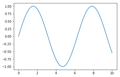
# plotting a line
x = np.linspace(0, 10, 100)
plt.plot(x, np.sin(x));
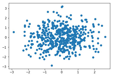
# scatter-plot points
x = np.random.normal(size=500)
y = np.random.normal(size=500)
plt.scatter(x, y);
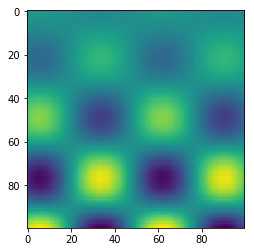
# showing images
x = np.linspace(1, 12, 100)
y = x[:, np.newaxis]

im = y * np.sin(x) * np.cos(y)
print(im.shape)
(100, 100)
# imshow - note that origin is at the top-left by default!
plt.imshow(im);
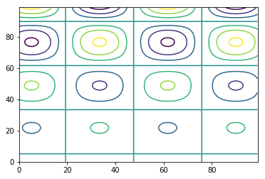
# Contour plot - note that origin here is at the bottom-left by default!
plt.contour(im);
There are many, many more plot types available. One useful way to explore these is by looking at the matplotlib gallery: http://matplotlib.org/gallery.html
You can test these examples out easily in the notebook: simply copy the
Source Code link on each page, and put it in a notebook using the
%load magic. For example:
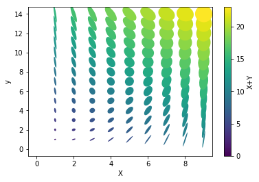
# %load http://matplotlib.org/mpl_examples/pylab_examples/ellipse_collection.py
import matplotlib.pyplot as plt
import numpy as np
from matplotlib.collections import EllipseCollection

x = np.arange(10)
y = np.arange(15)
X, Y = np.meshgrid(x, y)

XY = np.hstack((X.ravel()[:, np.newaxis], Y.ravel()[:, np.newaxis]))

ww = X/10.0
hh = Y/15.0
aa = X*9


fig, ax = plt.subplots()

ec = EllipseCollection(ww, hh, aa, units='x', offsets=XY,
                       transOffset=ax.transData)
ec.set_array((X + Y).ravel())
ax.add_collection(ec)
ax.autoscale_view()
ax.set_xlabel('X')
ax.set_ylabel('y')
cbar = plt.colorbar(ec)
cbar.set_label('X+Y');