2018-10-09 Ensemble, Gradient, Boosting…

Links: notebook, html, python, slides, GitHub

Le noteboook explore quelques particularités des algorithmes d’apprentissage pour expliquer certains résultats numériques. L’algoithme AdaBoost surpondère les exemples sur lequel un modèle fait des erreurs.

from jyquickhelper import add_notebook_menu
add_notebook_menu()

%matplotlib inline

Skewed split train test

Lorsqu’une classe est sous représentée, il est difficile de prédire les résultats d’un modèle de machine learning.

import numpy, numpy.random
from sklearn.model_selection import train_test_split
from sklearn.linear_model import LogisticRegression
from sklearn.tree import DecisionTreeClassifier
from sklearn.neural_network import MLPClassifier
from sklearn.ensemble import RandomForestClassifier, AdaBoostClassifier
from sklearn.metrics import confusion_matrix

N = 1000

res = []

for n in [1, 2, 5, 10, 20, 50, 80, 90, 100, 110]:
    print("n=", n)
    for k in range(10):

        X = numpy.zeros((N, 2))
        X[:, 0] = numpy.random.randint(0, 2, (N,))
        X[:, 1] = numpy.random.randint(0, n+1, (N,))
        Y = X[:, 0] + X[:, 1] + numpy.random.normal(size=(N,)) / 2
        Y[Y < 1.5] = 0
        Y[Y >= 1.5] = 1

        X_train, X_test, y_train, y_test = train_test_split(X, Y)

        stat = dict(N=N, n=n, ratio_train=y_train.sum()/y_train.shape[0],
                    k=k, ratio_test=y_test.sum()/y_test.shape[0])

        for model in [LogisticRegression(solver="liblinear"),
                      MLPClassifier(max_iter=500),
                      RandomForestClassifier(n_estimators=10),
                      AdaBoostClassifier(DecisionTreeClassifier(), n_estimators=10)]:
            obs = stat.copy()
            obs["model"] = model.__class__.__name__
            if obs["model"] == "AdaBoostClassifier":
                obs["model"] = "AdaB-" + model.base_estimator.__class__.__name__
            try:
                model.fit(X_train, y_train)
            except ValueError as e:
                obs["erreur"] = str(e)
                res.append(obs)
                continue
            sc = model.score(X_test, y_test)
            obs["accuracy"] = sc
            conf = confusion_matrix(y_test, model.predict(X_test))
            try:
                obs["Error-0|1"] = conf[0, 1] / conf[0, :].sum()
                obs["Error-1|0"] = conf[1, 0] / conf[1, :].sum()
            except Exception:
                pass
            res.append(obs)

n= 1
n= 2
n= 5
n= 10
n= 20
n= 50
n= 80
n= 90
n= 100
n= 110

from pandas import DataFrame
df = DataFrame(res)
df = df.sort_values(['n', 'model', 'model', "k"]).reset_index(drop=True)
df["diff_ratio"] = (df["ratio_test"] - df["ratio_train"]).abs()
df.head(n=5)

	N	n	ratio_train	k	ratio_test	model	accuracy	Error-0|1	Error-1|0	diff_ratio
0	1000	1	0.273333	0	0.300	AdaB-DecisionTreeClassifier	0.860	0.062857	0.320000	0.026667
1	1000	1	0.274667	1	0.328	AdaB-DecisionTreeClassifier	0.916	0.029762	0.195122	0.053333
2	1000	1	0.304000	2	0.284	AdaB-DecisionTreeClassifier	0.860	0.072626	0.309859	0.020000
3	1000	1	0.285333	3	0.268	AdaB-DecisionTreeClassifier	0.896	0.027322	0.313433	0.017333
4	1000	1	0.297333	4	0.256	AdaB-DecisionTreeClassifier	0.888	0.053763	0.281250	0.041333

df.tail(n=5)

	N	n	ratio_train	k	ratio_test	model	accuracy	Error-0|1	Error-1|0	diff_ratio
395	1000	110	0.982667	5	0.996	RandomForestClassifier	0.996	0.0	0.004016	0.013333
396	1000	110	0.990667	6	0.980	RandomForestClassifier	0.996	0.2	0.000000	0.010667
397	1000	110	0.985333	7	0.988	RandomForestClassifier	1.000	0.0	0.000000	0.002667
398	1000	110	0.985333	8	0.992	RandomForestClassifier	1.000	0.0	0.000000	0.006667
399	1000	110	0.985333	9	0.992	RandomForestClassifier	0.996	0.5	0.000000	0.006667

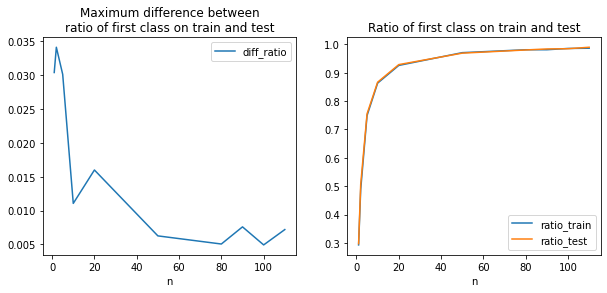
La répartition train/test est loin d’être statisfaisante lorsqu’il existe une classe sous représentée.

df[df.n==100][["n", "ratio_test", "ratio_train"]].head(n=10)

	n	ratio_test	ratio_train
320	100	0.980	0.992000
321	100	0.984	0.980000
322	100	0.988	0.984000
323	100	0.988	0.986667
324	100	0.976	0.986667
325	100	0.984	0.985333
326	100	0.984	0.981333
327	100	0.988	0.982667
328	100	0.984	0.989333
329	100	0.992	0.989333

#df.to_excel("data.xlsx")

columns = ["n", "N", "model"]
agg = df.groupby(columns, as_index=False).mean().sort_values(["n", "model"]).reset_index(drop=True)
agg.tail()

	n	N	model	ratio_train	k	ratio_test	accuracy	Error-0|1	Error-1|0	diff_ratio
35	100	1000	RandomForestClassifier	0.985733	4.5	0.9848	0.9956	0.185000	0.001216	0.004933
36	110	1000	AdaB-DecisionTreeClassifier	0.986533	4.5	0.9900	0.9972	0.130000	0.000810	0.007200
37	110	1000	LogisticRegression	0.986533	4.5	0.9900	0.9960	0.346667	0.000402	0.007200
38	110	1000	MLPClassifier	0.986533	4.5	0.9900	0.9956	0.346667	0.000810	0.007200
39	110	1000	RandomForestClassifier	0.986533	4.5	0.9900	0.9980	0.090000	0.000810	0.007200

import matplotlib.pyplot as plt
fig, ax = plt.subplots(1, 2, figsize=(10,4))
agg.plot(x="n", y="diff_ratio", ax=ax[0])
agg.plot(x="n", y="ratio_train", ax=ax[1])
agg.plot(x="n", y="ratio_test", ax=ax[1])
ax[0].set_title("Maximum difference between\nratio of first class on train and test")
ax[1].set_title("Ratio of first class on train and test")
ax[0].legend();

Une astuce pour éviter les doublons avant d’effecturer un pivot.

agg2 = agg.copy()
agg2["ratio_test2"] = agg2["ratio_test"] + agg2["n"] / 100000

import matplotlib.pyplot as plt
fig, ax = plt.subplots(1, 3, figsize=(14,4))
agg2.pivot("ratio_test2", "model", "accuracy").plot(ax=ax[0])
agg2.pivot("ratio_test2", "model", "Error-0|1").plot(ax=ax[1])
agg2.pivot("ratio_test2", "model", "Error-1|0").plot(ax=ax[2])
ax[0].plot([0.5, 1.0], [0.5, 1.0], '--', label="constant")
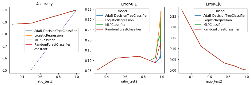
ax[0].set_title("Accuracy")
ax[1].set_title("Error-0|1")
ax[2].set_title("Error-1|0")
ax[0].legend();

agg2.pivot("ratio_test2", "model", "Error-0|1")

model	AdaB-DecisionTreeClassifier	LogisticRegression	MLPClassifier	RandomForestClassifier
ratio_test2
0.29721	0.052249	0.052249	0.052249	0.052249
0.50682	0.110686	0.110686	0.110686	0.110686
0.75525	0.119578	0.119578	0.119578	0.119578
0.86690	0.099333	0.099333	0.099333	0.099333
0.92900	0.088095	0.113095	0.113095	0.088095
0.96970	0.106349	0.253968	0.220635	0.163492
0.98120	0.125000	0.310000	0.200000	0.175000
0.98490	0.110000	0.155000	0.155000	0.170000
0.98580	0.185000	0.335000	0.268333	0.185000
0.99110	0.130000	0.346667	0.346667	0.090000

Le modèle AdaBoost construit 10 arbres tout comme la forêt aléatoire à ceci près que le poids associé à chacun des arbres des différents et non uniforme.

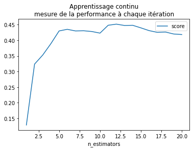
Apprentissage continu

Apprendre une forêt aléatoire, puis ajouter un arbre, encore un tout en gardant le résultat des apprentissages précédents.

from sklearn.datasets import load_diabetes
data = load_diabetes()
X, y = data.data, data.target

X_train, X_test, y_train, y_test = train_test_split(X, y)

from sklearn.ensemble import RandomForestRegressor

model = None
res = []
for i in range(0, 20):
    if model is None:
        model = RandomForestRegressor(n_estimators=1, warm_start=True)
    else:
        model.set_params(**dict(n_estimators=model.n_estimators+1))
    model.fit(X_train, y_train)
    score = model.score(X_test, y_test)
    res.append(dict(n_estimators=model.n_estimators, score=score))

df = DataFrame(res)
df.head()

	n_estimators	score
0	1	0.128906
1	2	0.323854
2	3	0.352876
3	4	0.389476
4	5	0.429992

ax = df.plot(x="n_estimators", y="score")
ax.set_title("Apprentissage continu\nmesure de la performance à chaque itération");