2A.ml - Statistiques descriptives avec scikit-learn - correction#

Links: notebook, html, python, slides, GitHub

ACP, CAH, régression linéaire, correction.

%matplotlib inline

import matplotlib.pyplot as plt

from jyquickhelper import add_notebook_menu
add_notebook_menu()

# Répare une incompatibilité entre scipy 1.0 et statsmodels 0.8.
from pymyinstall.fix import fix_scipy10_for_statsmodels08
fix_scipy10_for_statsmodels08()

Prérequis de l’énoncé #

import pyensae.datasource
f = pyensae.datasource.download_data("dads2011_gf_salaries11_dbase.zip",
                          website="https://www.insee.fr/fr/statistiques/fichier/2011542/")

import pandas
try:
    from dbfread import DBF
    use_dbfread = True
except ImportError as e :
    use_dbfread = False

if use_dbfread:
    import os
    from pyensae.sql.database_exception import ExceptionSQL
    from pyensae.datasource import dBase2sqllite
    print("convert dbase into sqllite")
    try:
        dBase2sqllite("salaries2011.db3", "varlist_salaries11.dbf", overwrite_table="varlist")
        dBase2sqllite("salaries2011.db3", "varmod_salaries11.dbf", overwrite_table="varmod")
        dBase2sqllite("salaries2011.db3", 'salaries11.dbf', overwrite_table="salaries", fLOG = print)
    except ExceptionSQL:
        print("La base de données est déjà renseignée.")
else :
    print("use of zipped version")
    import pyensae.datasource
    db3 = pyensae.datasource.download_data("salaries2011.zip")
    # pour aller plus vite, données à télécharger au
    # http://www.xavierdupre.fr/enseignement/complements/salaries2011.zip

convert dbase into sqllite
unable to execute a SQL request (1)(file salaries2011.db3)
create table varlist (VARIABLE TEXT, LIBELLE TEXT, TYPE TEXT, LONGUEUR REAL)
La base de données est déjà renseignée.

Exercice 1 : CAH (classification ascendante hiérarchique)#

Le point commun de ces méthodes est qu’elles ne sont pas supervisées. L’objectif est de réduire la complexité des données. Réduire le nombre de dimensions pour l’ACP ou segmenter les observations pour les k-means et la CAH.

import pandas, numpy, matplotlib.pyplot as plt
from sklearn.decomposition import PCA
import pyensae.datasource

pyensae.datasource.download_data("eleve_region.txt")
df = pandas.read_csv("eleve_region.txt", sep="\t", encoding="utf8", index_col=0)
print(df.shape)
df.head(n=5)

(27, 21)

	1993	1994	1995	1996	1997	1998	1999	2000	2001	2002	...	2004	2005	2006	2007	2008	2009	2010	2011	2012	2013
académie
Aix-Marseille	241357	242298	242096	242295	243660	244608	245536	247288	249331	250871	...	250622	248208	245755	243832	242309	240664	240432	241336	239051	240115
Amiens	198281	196871	195709	194055	192893	191862	189636	185977	183357	180973	...	175610	172110	168718	165295	163116	162548	163270	164422	165275	166345
Besançon	116373	115600	114282	113312	112076	110261	108106	105463	103336	102264	...	100117	98611	97038	95779	95074	94501	94599	94745	94351	94613
Bordeaux	253551	252644	249658	247708	247499	245757	244992	243047	243592	245198	...	244805	244343	242602	242933	243146	244336	246806	250626	252085	255761
Caen	145435	144369	141883	140658	139585	137704	135613	133255	131206	129271	...	125552	123889	122550	121002	119857	119426	119184	119764	119010	119238

5 rows × 21 columns

for c in df.columns:
    if c != "1993":
        df[c] /= df ["1993"]
df["1993"] /= df["1993"]
df.head()

	1993	1994	1995	1996	1997	1998	1999	2000	2001	2002	...	2004	2005	2006	2007	2008	2009	2010	2011	2012	2013
académie
Aix-Marseille	1.0	1.003899	1.003062	1.003886	1.009542	1.013470	1.017315	1.024574	1.033038	1.039419	...	1.038387	1.028385	1.018222	1.010255	1.003944	0.997129	0.996168	0.999913	0.990446	0.994854
Amiens	1.0	0.992889	0.987029	0.978687	0.972826	0.967627	0.956400	0.937947	0.924733	0.912710	...	0.885662	0.868011	0.850904	0.833640	0.822651	0.819786	0.823427	0.829237	0.833539	0.838936
Besançon	1.0	0.993358	0.982032	0.973697	0.963076	0.947479	0.928961	0.906250	0.887972	0.878761	...	0.860311	0.847370	0.833853	0.823035	0.816976	0.812053	0.812895	0.814149	0.810764	0.813015
Bordeaux	1.0	0.996423	0.984646	0.976955	0.976131	0.969261	0.966243	0.958572	0.960722	0.967056	...	0.965506	0.963684	0.956817	0.958123	0.958963	0.963656	0.973398	0.988464	0.994218	1.008716
Caen	1.0	0.992670	0.975577	0.967154	0.959776	0.946842	0.932465	0.916251	0.902162	0.888858	...	0.863286	0.851851	0.842644	0.832001	0.824128	0.821164	0.819500	0.823488	0.818304	0.819871

5 rows × 21 columns

from sklearn.cluster import AgglomerativeClustering

ward = AgglomerativeClustering(linkage='ward', compute_full_tree=True).fit(df)
ward

AgglomerativeClustering(compute_full_tree=True)

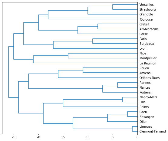
from scipy.cluster.hierarchy import dendrogram
import matplotlib.pyplot as plt

dendro = [ ]
for a,b in ward.children_:
    dendro.append([a, b, float(len(dendro)+1), len(dendro)+1])
    # le dernier coefficient devrait contenir le nombre de feuilles dépendant de ce noeud
    # et non le dernier indice
    # de même, le niveau (3ème colonne) ne devrait pas être le nombre de noeud
    # mais la distance de Ward

fig = plt.figure( figsize=(8,8) )
ax = fig.add_subplot(1,1,1)
r = dendrogram(dendro, color_threshold=1, labels=list(df.index),
               show_leaf_counts=True, ax=ax, orientation="left")

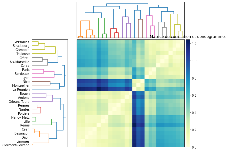
../_images/td2a_correction_session_3A_11_0.png

Je reprends également le graphique montrant la matrice de corrélations qu’on peut également obtenir avec seaborn : clustermap.

from scipy.spatial.distance import pdist, squareform

data_dist = pdist(df)

fig = plt.figure(figsize=(8,8))

# x ywidth height
ax1 = fig.add_axes([0.05,0.1,0.2,0.6])
Z1 = dendrogram(dendro, orientation='right',labels=list(df.index))
ax1.set_xticks([])

# Compute and plot second dendrogram.
ax2 = fig.add_axes([0.3,0.71,0.6,0.2])
Z2 = dendrogram(dendro)
ax2.set_xticks([])
ax2.set_yticks([])

# Compute and plot the heatmap
axmatrix = fig.add_axes([0.3,0.1,0.6,0.6])
idx1 = Z1['leaves']
idx2 = Z2['leaves']

D = squareform(data_dist)
D = D[idx1,:]
D = D[:,idx2]
im = axmatrix.matshow(D, aspect='auto', origin='lower', cmap=plt.cm.YlGnBu)
axmatrix.set_xticks([])
axmatrix.set_yticks([])

# Plot colorbar.
axcolor = fig.add_axes([0.91,0.1,0.02,0.6])
plt.colorbar(im, cax=axcolor)
plt.title("Matrice de corrélation et dendogramme.");

../_images/td2a_correction_session_3A_13_0.png

Exercice 2 : régression linéaire #

Ce sont trois méthodes supervisées : on s’en sert pour expliquer prédire le lien entre deux variables $X$ et $Y$ (ou ensemble de variables) ou prédire $Y$ en fonction de $X$ . On suppose que les données ont déjà été téléchargées (voir l’énoncé de cet exercice). On continue avec l’extraction de l’âge, du sexe et du salaire comme indiqué dans l’énoncé.

import sqlite3, pandas
con = sqlite3.connect("salaries2011.db3")
df = pandas.io.sql.read_sql("select * from varmod", con)
con.close()

values = df[ df.VARIABLE == "TRNNETO"].copy()

def process_intervalle(s):
    # [14 000 ; 16 000[ euros
    acc = "0123456789;+"
    s0 = "".join(c for c in s if c in acc)
    spl = s0.split(';')
    if len(spl) != 2:
        raise ValueError("Unable to process '{0}'".format(s0))
    try:
        a = float(spl[0])
    except Exception as e:
        raise ValueError("Cannot interpret '{0}' - {1}".format(s, spl))
    b = float(spl[1]) if "+" not in spl[1] else None
    if b is None:
        return a
    return (a+b) / 2.0

values["montant"] = values.apply(lambda r : process_intervalle(r["MODLIBELLE"]), axis=1)
values.head()

	VARIABLE	MODALITE	MODLIBELLE	montant
8957	TRNNETO	00	[0 ; 200[ euros	100.0
8958	TRNNETO	01	[200 ; 500[ euros	350.0
8959	TRNNETO	02	[500 ; 1 000[ euros	750.0
8960	TRNNETO	03	[1 000 ; 1 500[ euros	1250.0
8961	TRNNETO	04	[1 500 ; 2 000[ euros	1750.0

import sqlite3, pandas
con = sqlite3.connect("salaries2011.db3")
data = pandas.io.sql.read_sql("select TRNNETO,AGE,SEXE from salaries", con)
con.close()

salaires = data.merge (values, left_on="TRNNETO", right_on="MODALITE" )
salaires["M"] = salaires.apply(lambda r: 1 if r["SEXE"] == "1" else 0, axis=1)
salaires["F"] = salaires.apply(lambda r: 1 if r["SEXE"] == "2" else 0, axis=1)
data = salaires[["AGE","M","F","montant"]]
data = data [data.M + data.F > 0]
data.head()

	AGE	M	F	montant
0	49.0	1	0	750.0
1	27.0	1	0	750.0
2	22.0	1	0	750.0
3	26.0	1	0	750.0
4	29.0	0	1	750.0

On supprime les valeurs manquantes :

nonull = data.dropna().copy()
nonull.shape

(2240691, 4)

version scikit-learn #

La régression linéraire suit :

nonull[["AGE","M"]].dropna().shape

(2240691, 2)

from sklearn import linear_model
clf = linear_model.LinearRegression()
clf.fit (nonull[["AGE","M"]].values, nonull.montant.values)
clf.coef_, clf.intercept_, "R^2=", clf.score(
    nonull[["AGE","M"]], nonull.montant)

C:Python395_x64libsite-packagessklearnbase.py:443: UserWarning: X has feature names, but LinearRegression was fitted without feature names
  warnings.warn(

(array([ 310.98873096, 4710.02901965]),
 4927.219006697269,
 'R^2=',
 0.13957345814666222)

On prend un échantillon aléatoire :

import random
val = nonull.copy()
val["rnd"] = val.apply(lambda r: random.randint(0, 1000), axis=1)
ech = val[val["rnd"] == 1]
ech.shape

(2278, 5)

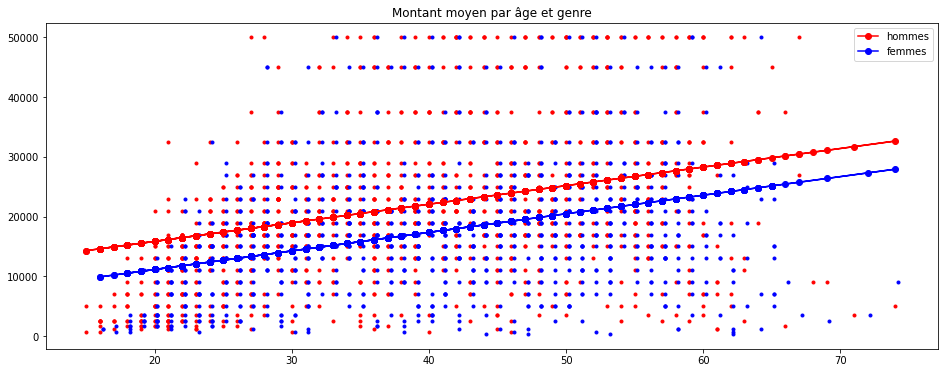
On sépare homme et femmes :

homme = ech[ech.M == 1]
femme = ech[ech.M == 0]

predh = clf.predict(homme[["AGE","M"]])
predf = clf.predict(femme[["AGE","M"]])

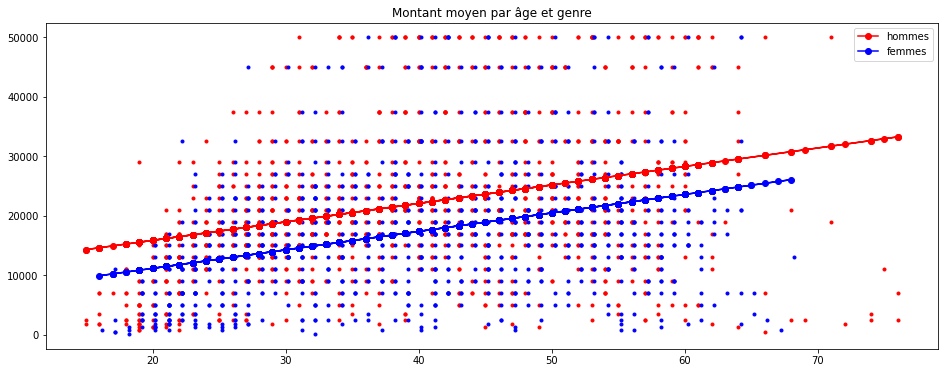
import matplotlib.pyplot as plt
plt.figure(figsize=(16,6))
plt.plot(homme.AGE, homme.montant, "r.")
plt.plot(femme.AGE + 0.2, femme.montant, "b.")
plt.plot(homme.AGE, predh, "ro-", label="hommes")
plt.plot(femme.AGE, predf, "bo-", label="femmes")
plt.legend()
plt.title("Montant moyen par âge et genre");

C:Python395_x64libsite-packagessklearnbase.py:443: UserWarning: X has feature names, but LinearRegression was fitted without feature names
  warnings.warn(
C:Python395_x64libsite-packagessklearnbase.py:443: UserWarning: X has feature names, but LinearRegression was fitted without feature names
  warnings.warn(

../_images/td2a_correction_session_3A_25_1.png

version statsmodels #

import statsmodels.api as sm
nonull["one"] = 1.0  # on ajoute la constante
model = sm.OLS(nonull.montant, nonull [["AGE","M", "one"]])
results = model.fit()
print("coefficients",results.params)
results.summary()

C:Python395_x64libsite-packagesstatsmodelstsabasetsa_model.py:7: FutureWarning: pandas.Int64Index is deprecated and will be removed from pandas in a future version. Use pandas.Index with the appropriate dtype instead.
  from pandas import (to_datetime, Int64Index, DatetimeIndex, Period,
C:Python395_x64libsite-packagesstatsmodelstsabasetsa_model.py:7: FutureWarning: pandas.Float64Index is deprecated and will be removed from pandas in a future version. Use pandas.Index with the appropriate dtype instead.
  from pandas import (to_datetime, Int64Index, DatetimeIndex, Period,

coefficients AGE     310.988731
M      4710.029020
one    4927.219007
dtype: float64

OLS Regression Results
Dep. Variable:	montant	R-squared:	0.140
Model:	OLS	Adj. R-squared:	0.140
Method:	Least Squares	F-statistic:	1.817e+05
Date:	Sat, 12 Feb 2022	Prob (F-statistic):	0.00
Time:	18:57:08	Log-Likelihood:	-2.4023e+07
No. Observations:	2240691	AIC:	4.805e+07
Df Residuals:	2240688	BIC:	4.805e+07
Df Model:	2
Covariance Type:	nonrobust

	coef	std err	t	P>\|t\|	[0.025	0.975]
AGE	310.9887	0.600	518.682	0.000	309.814	312.164
M	4710.0290	14.658	321.323	0.000	4681.299	4738.759
one	4927.2190	26.032	189.272	0.000	4876.196	4978.242

Omnibus:	132298.944	Durbin-Watson:	0.183
Prob(Omnibus):	0.000	Jarque-Bera (JB):	158649.997
Skew:	0.614	Prob(JB):	0.00
Kurtosis:	3.440	Cond. No.	150.

Notes:
[1] Standard Errors assume that the covariance matrix of the errors is correctly specified.

On reproduit le même dessin :

import random
val = nonull.copy()
val["rnd"] = val.apply(lambda r: random.randint(0,1000), axis=1)
ech = val[val["rnd"] == 1]

homme = ech [ ech.M == 1]
femme = ech [ ech.M == 0]

predh = results.predict(homme[["AGE","M","one"]])
predf = results.predict(femme[["AGE","M","one"]])

import matplotlib.pyplot as plt
def graph(homme, femme, predh, predf):
    fig, ax = plt.subplots(1, 1, figsize=(16, 6))
    ax.plot(homme.AGE, homme.montant, "r.")
    ax.plot(femme.AGE + 0.2, femme.montant, "b.")
    ax.plot(homme.AGE, predh, "ro-", label="hommes")
    ax.plot(femme.AGE, predf, "bo-", label="femmes")
    ax.legend()
    ax.set_title("Montant moyen par âge et genre");
    return ax

graph(homme, femme, predh, predf);

../_images/td2a_correction_session_3A_30_0.png

On ajoute l’intervalle de confiance sur un échantillon :

from statsmodels.sandbox.regression.predstd import wls_prediction_std

prstd, iv_l, iv_u = wls_prediction_std(results)

val = nonull.copy()
val["rnd"] = val.apply(lambda r: random.randint(0, 1000), axis=1)
val["pred"] = prstd
val["up"] = iv_u
val["down"] = iv_l

ech = val[val["rnd"] == 1]
ech.head()

	AGE	M	F	montant	one	rnd	pred	up	down
86	34.0	0	1	750.0	1.0	1	10964.546920	36990.964539	-5989.292820
355	48.0	0	1	750.0	1.0	1	10964.547492	41344.807893	-1635.451707
1046	68.0	0	1	750.0	1.0	1	10964.559457	47564.605962	4584.299462
2008	21.0	0	1	750.0	1.0	1	10964.552144	32948.121273	-10032.156559
3761	18.0	1	0	750.0	1.0	1	10964.553468	36725.186695	-6255.096328

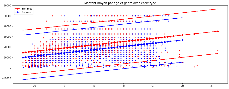
Puis on l’ajoute au graphe précédent :

homme = ech[ech.M == 1]
femme = ech[ech.M == 0]

predh = results.predict(homme[["AGE","M","one"]])
predf = results.predict(femme[["AGE","M","one"]])

ax = graph(homme, femme, predh, predf)
ax.plot(homme.AGE, homme.up, 'r-')
ax.plot(homme.AGE, homme.down, 'r-')
ax.plot(femme.AGE, femme.up, 'b-')
ax.plot(femme.AGE, femme.down, 'b-')
ax.set_title("Montant moyen par âge et genre avec écart-type");

../_images/td2a_correction_session_3A_34_0.png

Liens

Contenu

Information

Sujet précédent

Sujet suivant

2A.ml - Statistiques descriptives avec scikit-learn - correction#

Prérequis de l’énoncé #

Exercice 1 : CAH (classification ascendante hiérarchique)#

Exercice 2 : régression linéaire #

version scikit-learn #

version statsmodels #

Liens

Contenu

Information

Sujet précédent

Sujet suivant

2A.ml - Statistiques descriptives avec scikit-learn - correction#

Prérequis de l’énoncé#

Exercice 1 : CAH (classification ascendante hiérarchique)#

Exercice 2 : régression linéaire#

version scikit-learn#

version statsmodels#

Prérequis de l’énoncé #

Exercice 2 : régression linéaire #

version scikit-learn #

version statsmodels #