2A.ml - Réduction d’une forêt aléatoire - correction#
Links: notebook, html, python, slides, GitHub
Le modèle Lasso permet de sélectionner des variables, une forêt aléatoire produit une prédiction comme étant la moyenne d’arbres de régression. Et si on mélangeait les deux ?
from jyquickhelper import add_notebook_menu
add_notebook_menu()
%matplotlib inline
Datasets#
Comme il faut toujours des données, on prend ce jeu Diabetes.
from sklearn.datasets import load_diabetes
data = load_diabetes()
X, y = data.data, data.target
from sklearn.model_selection import train_test_split
X_train, X_test, y_train, y_test = train_test_split(X, y)
Une forêt aléatoire#
from sklearn.ensemble import RandomForestRegressor as model_class
clr = model_class()
clr.fit(X_train, y_train)
RandomForestRegressor()In a Jupyter environment, please rerun this cell to show the HTML representation or trust the notebook.
On GitHub, the HTML representation is unable to render, please try loading this page with nbviewer.org.
RandomForestRegressor()
Le nombre d’arbres est…
len(clr.estimators_)
100
from sklearn.metrics import r2_score
r2_score(y_test, clr.predict(X_test))
0.3625404922781166
Random Forest = moyenne des prédictions#
On recommence en faisant la moyenne soi-même.
import numpy
dest = numpy.zeros((X_test.shape[0], len(clr.estimators_)))
estimators = numpy.array(clr.estimators_).ravel()
for i, est in enumerate(estimators):
    pred = est.predict(X_test)
    dest[:, i] = pred

average = numpy.mean(dest, axis=1)
r2_score(y_test, average)
0.3625404922781166
A priori, c’est la même chose.
Pondérer les arbres à l’aide d’une régression linéaire#
La forêt aléatoire est une façon de créer de nouvelles features, 100 exactement qu’on utilise pour caler une régression linéaire.
from sklearn.linear_model import LinearRegression


def new_features(forest, X):
    dest = numpy.zeros((X.shape[0], len(forest.estimators_)))
    estimators = numpy.array(forest.estimators_).ravel()
    for i, est in enumerate(estimators):
        pred = est.predict(X)
        dest[:, i] = pred
    return dest


X_train_2 = new_features(clr, X_train)
lr = LinearRegression()
lr.fit(X_train_2, y_train)
LinearRegression()In a Jupyter environment, please rerun this cell to show the HTML representation or trust the notebook.
On GitHub, the HTML representation is unable to render, please try loading this page with nbviewer.org.
LinearRegression()
X_test_2 = new_features(clr, X_test)
r2_score(y_test, lr.predict(X_test_2))
0.30414556638121215
Un peu moins bien, un peu mieux, le risque d’overfitting est un peu plus
grand avec ces nombreuses features car la base d’apprentissage ne
contient que 379 observations (regardez X_train.shape pour
vérifier).
lr.coef_
array([ 0.0129567 , -0.03467343, -0.02574902,  0.01872549,  0.00128276,
       -0.01449147,  0.00977528, -0.02397026,  0.01066261,  0.02121925,
        0.03544455,  0.02735311,  0.01859875, -0.03189411, -0.0245749 ,
       -0.01879966,  0.01521987,  0.00292998,  0.04250576,  0.01424533,
       -0.00561623,  0.00635399,  0.04712406,  0.02518721,  0.01713507,
        0.01741708, -0.02072389,  0.05748854,  0.00424951,  0.02872275,
       -0.01016485,  0.04368062,  0.07377962,  0.06540726, -0.00123185,
        0.02227104,  0.0289425 ,  0.00914512,  0.03645644,  0.01838009,
        0.00046509,  0.04145444,  0.0202303 ,  0.00984027,  0.0149448 ,
       -0.01129977,  0.00428108,  0.02601842,  0.00421449, -0.01172942,
        0.02631074,  0.04180424,  0.02909078, -0.01922766, -0.00953341,
       -0.0036882 , -0.02411783,  0.06700977, -0.01447105,  0.02094102,
        0.00227497,  0.04181756, -0.02474879,  0.0465355 ,  0.05504502,
       -0.05645067, -0.02066304,  0.04349629, -0.01549704,  0.02805018,
        0.01344701,  0.03489881,  0.04401519,  0.04756385, -0.02936105,
       -0.0305603 , -0.02101141,  0.02751049, -0.00875684, -0.01583926,
        0.00033533,  0.02769942,  0.0358323 , -0.04180737, -0.02759142,
       -0.01231979,  0.02881228, -0.00406825,  0.00497993,  0.01094388,
       -0.01672934,  0.05414844, -0.01725494,  0.04816335,  0.04487341,
        0.0269151 ,  0.00945554,  0.02318397,  0.04105411,  0.05314256])
import matplotlib.pyplot as plt
fig, ax = plt.subplots(1, 1, figsize=(12, 4))
ax.bar(numpy.arange(0, len(lr.coef_)), lr.coef_)
ax.set_title("Coefficients pour chaque arbre calculés avec une régression linéaire");
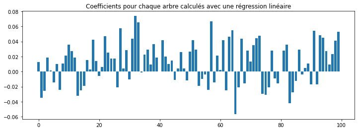
Le score est avec une régression linéaire sur les variables initiales est nettement moins élevé.
lr_raw = LinearRegression()
lr_raw.fit(X_train, y_train)
r2_score(y_test, lr_raw.predict(X_test))
0.5103612609676136
Sélection d’arbres#
L’idée est d’utiliser un algorithme de sélection de variables type Lasso pour réduire la forêt aléatoire sans perdre en performance. C’est presque le même code.
from sklearn.linear_model import Lasso

lrs = Lasso(max_iter=10000)
lrs.fit(X_train_2, y_train)
lrs.coef_
array([ 0.01256934, -0.03342528, -0.02400605,  0.01825851,  0.0005323 ,
       -0.01374509,  0.01004616, -0.02284903,  0.01105419,  0.02047233,
        0.03476362,  0.02755575,  0.01751674, -0.03051477, -0.02321124,
       -0.01783216,  0.01429992,  0.00214398,  0.04066576,  0.0134879 ,
       -0.00377705,  0.00506043,  0.04614375,  0.02482044,  0.01560689,
        0.01706262, -0.02035898,  0.05747191,  0.00418486,  0.02766988,
       -0.00899098,  0.04325266,  0.07327657,  0.06515135, -0.00034774,
        0.02210777,  0.0280344 ,  0.00852669,  0.0358763 ,  0.01779845,
        0.        ,  0.03970822,  0.01935286,  0.00908017,  0.01417323,
       -0.01066044,  0.00293442,  0.02483663,  0.00332255, -0.01043329,
        0.02666477,  0.04097776,  0.02851599, -0.01795373, -0.00830115,
       -0.00293032, -0.02188798,  0.06679156, -0.01364001,  0.02028321,
        0.00160792,  0.04114419, -0.02342478,  0.04638246,  0.0547764 ,
       -0.05501755, -0.01856303,  0.04157578, -0.01403205,  0.02718244,
        0.01215738,  0.03503149,  0.04403975,  0.04640854, -0.02884553,
       -0.02929629, -0.01946676,  0.02679733, -0.00779812, -0.01418256,
        0.        ,  0.02734732,  0.03608281, -0.04111661, -0.02654714,
       -0.01106999,  0.02664032, -0.00291639,  0.00541073,  0.01187597,
       -0.01621428,  0.05386765, -0.01531834,  0.04807872,  0.04398675,
        0.02611443,  0.00944403,  0.02219076,  0.04080548,  0.05276076])
Pas mal de zéros donc pas mal d’arbres non utilisés.
r2_score(y_test, lrs.predict(X_test_2))
0.3055529526371402
Pas trop de perte… Ca donne envie d’essayer plusieurs valeur de
alpha.
from tqdm import tqdm
alphas = [0.01 * i for i in range(100)] +[1 + 0.1 * i for i in range(100)]
obs = []
for i in tqdm(range(0, len(alphas))):
    alpha = alphas[i]
    lrs = Lasso(max_iter=20000, alpha=alpha)
    lrs.fit(X_train_2, y_train)
    obs.append(dict(
        alpha=alpha,
        null=len(lrs.coef_[lrs.coef_!=0]),
        r2=r2_score(y_test, lrs.predict(X_test_2))
    ))
  0%|          | 0/200 [00:00<?, ?it/s]C:UsersxavieAppDataLocalTempipykernel_182521667502338.py:7: UserWarning: With alpha=0, this algorithm does not converge well. You are advised to use the LinearRegression estimator
  lrs.fit(X_train_2, y_train)
C:xavierdupre__home_github_forkscikit-learnsklearnlinear_model_coordinate_descent.py:634: UserWarning: Coordinate descent with no regularization may lead to unexpected results and is discouraged.
  model = cd_fast.enet_coordinate_descent(
C:xavierdupre__home_github_forkscikit-learnsklearnlinear_model_coordinate_descent.py:634: ConvergenceWarning: Objective did not converge. You might want to increase the number of iterations, check the scale of the features or consider increasing regularisation. Duality gap: 3.572e+04, tolerance: 1.993e+02 Linear regression models with null weight for the l1 regularization term are more efficiently fitted using one of the solvers implemented in sklearn.linear_model.Ridge/RidgeCV instead.
  model = cd_fast.enet_coordinate_descent(
100%|██████████| 200/200 [00:37<00:00,  5.37it/s]
from pandas import DataFrame
df = DataFrame(obs)
df.tail()
| alpha | null | r2 | |
|---|---|---|---|
| 195 | 10.5 | 83 | 0.318660 |
| 196 | 10.6 | 83 | 0.318771 |
| 197 | 10.7 | 83 | 0.318879 |
| 198 | 10.8 | 83 | 0.318982 |
| 199 | 10.9 | 82 | 0.319073 |
fig, ax = plt.subplots(1, 2, figsize=(12, 4))
df[["alpha", "null"]].set_index("alpha").plot(ax=ax[0], logx=True)
ax[0].set_title("Nombre de coefficients non nulls")
df[["alpha", "r2"]].set_index("alpha").plot(ax=ax[1], logx=True)
ax[1].set_title("r2");
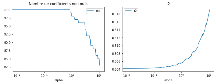
Dans ce cas, supprimer des arbres augmente la performance, comme évoqué ci-dessus, cela réduit l’overfitting. Le nombre d’arbres peut être réduit des deux tiers avec ce modèle.