Piecewise linear regression with scikit-learn predictors

Links: notebook, html, PDF, python, slides, GitHub

The notebook illustrates an implementation of a piecewise linear regression based on scikit-learn. The bucketization can be done with a DecisionTreeRegressor or a KBinsDiscretizer. A linear model is then fitted on each bucket.

from jyquickhelper import add_notebook_menu
add_notebook_menu()

%matplotlib inline

import warnings
warnings.simplefilter("ignore")

Piecewise data

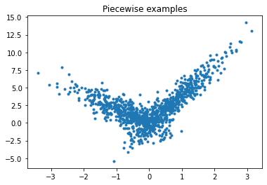
Let’s build a toy problem based on two linear models.

import numpy
import numpy.random as npr
X = npr.normal(size=(1000,4))
alpha = [4, -2]
t = (X[:, 0] + X[:, 3] * 0.5) > 0
switch = numpy.zeros(X.shape[0])
switch[t] = 1
y = alpha[0] * X[:, 0] * t + alpha[1] * X[:, 0] * (1-t) + X[:, 2]

import matplotlib.pyplot as plt
fig, ax = plt.subplots(1, 1)
ax.plot(X[:, 0], y, ".")
ax.set_title("Piecewise examples");

Piecewise Linear Regression with a decision tree

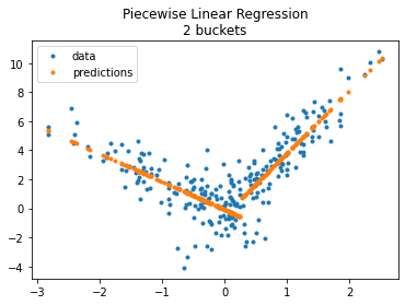
The first example is done with a decision tree.

from sklearn.model_selection import train_test_split
X_train, X_test, y_train, y_test = train_test_split(X[:, :1], y)

from mlinsights.mlmodel import PiecewiseRegressor
from sklearn.tree import DecisionTreeRegressor

model = PiecewiseRegressor(verbose=True,
                           binner=DecisionTreeRegressor(min_samples_leaf=300))
model.fit(X_train, y_train)

[Parallel(n_jobs=1)]: Using backend SequentialBackend with 1 concurrent workers.
[Parallel(n_jobs=1)]: Done   2 out of   2 | elapsed:    0.0s finished

PiecewiseRegressor(binner=DecisionTreeRegressor(min_samples_leaf=300),
                   estimator=LinearRegression(), verbose=True)

pred = model.predict(X_test)
pred[:5]

array([0.38877424, 2.59190533, 0.96242534, 3.40015406, 1.20811239])

fig, ax = plt.subplots(1, 1)
ax.plot(X_test[:, 0], y_test, ".", label='data')
ax.plot(X_test[:, 0], pred, ".", label="predictions")
ax.set_title("Piecewise Linear Regression\n2 buckets")
ax.legend();

The method transform_bins returns the bucket of each variables, the final leave from the tree.

model.transform_bins(X_test)

array([0., 1., 0., 1., 1., 0., 0., 1., 0., 1., 0., 0., 1., 1., 1., 1., 0.,
       0., 1., 1., 0., 1., 0., 0., 0., 0., 1., 1., 1., 0., 0., 1., 1., 0.,
       1., 0., 1., 0., 0., 0., 1., 0., 1., 1., 1., 0., 0., 0., 0., 1., 0.,
       1., 0., 0., 0., 1., 0., 0., 0., 1., 0., 0., 1., 1., 0., 1., 0., 0.,
       0., 1., 1., 1., 1., 0., 0., 1., 0., 0., 0., 0., 1., 0., 1., 0., 0.,
       0., 1., 1., 0., 0., 1., 0., 0., 1., 0., 0., 0., 0., 1., 1., 0., 0.,
       1., 0., 1., 0., 1., 0., 0., 1., 0., 1., 0., 1., 1., 1., 0., 0., 1.,
       0., 1., 0., 0., 0., 0., 1., 0., 1., 0., 0., 1., 1., 0., 1., 0., 0.,
       0., 0., 0., 1., 1., 1., 0., 0., 1., 0., 0., 1., 0., 1., 0., 0., 0.,
       0., 1., 0., 1., 1., 0., 1., 0., 0., 0., 0., 0., 0., 0., 0., 1., 1.,
       1., 0., 0., 0., 1., 0., 1., 1., 1., 1., 0., 0., 0., 1., 0., 1., 1.,
       1., 1., 0., 0., 0., 0., 0., 1., 0., 0., 1., 1., 1., 0., 0., 0., 1.,
       0., 1., 0., 0., 0., 0., 0., 0., 1., 0., 1., 0., 0., 0., 1., 0., 1.,
       1., 1., 0., 1., 0., 1., 1., 1., 0., 0., 0., 1., 0., 0., 0., 0., 0.,
       1., 0., 1., 0., 1., 0., 1., 0., 0., 1., 1., 1.])

Let’s try with more buckets.

model = PiecewiseRegressor(verbose=False,
                           binner=DecisionTreeRegressor(min_samples_leaf=150))
model.fit(X_train, y_train)

PiecewiseRegressor(binner=DecisionTreeRegressor(min_samples_leaf=150),
                   estimator=LinearRegression())

import matplotlib.pyplot as plt
fig, ax = plt.subplots(1, 1)
ax.plot(X_test[:, 0], y_test, ".", label='data')
ax.plot(X_test[:, 0], model.predict(X_test), ".", label="predictions")
ax.set_title("Piecewise Linear Regression\n4 buckets")
ax.legend();

Piecewise Linear Regression with a KBinsDiscretizer

from sklearn.preprocessing import KBinsDiscretizer

model = PiecewiseRegressor(verbose=True,
                           binner=KBinsDiscretizer(n_bins=2))
model.fit(X_train, y_train)

[Parallel(n_jobs=1)]: Using backend SequentialBackend with 1 concurrent workers.
[Parallel(n_jobs=1)]: Done   2 out of   2 | elapsed:    0.0s finished

PiecewiseRegressor(binner=KBinsDiscretizer(n_bins=2),
                   estimator=LinearRegression(), verbose=True)

fig, ax = plt.subplots(1, 1)
ax.plot(X_test[:, 0], y_test, ".", label='data')
ax.plot(X_test[:, 0], model.predict(X_test), ".", label="predictions")
ax.set_title("Piecewise Linear Regression\n2 buckets")
ax.legend();

model = PiecewiseRegressor(verbose=True,
                           binner=KBinsDiscretizer(n_bins=4))
model.fit(X_train, y_train)

[Parallel(n_jobs=1)]: Using backend SequentialBackend with 1 concurrent workers.
[Parallel(n_jobs=1)]: Done   4 out of   4 | elapsed:    0.0s finished

PiecewiseRegressor(binner=KBinsDiscretizer(n_bins=4),
                   estimator=LinearRegression(), verbose=True)

fig, ax = plt.subplots(1, 1)
ax.plot(X_test[:, 0], y_test, ".", label='data')
ax.plot(X_test[:, 0], model.predict(X_test), ".", label="predictions")
ax.set_title("Piecewise Linear Regression\n4 buckets")
ax.legend();

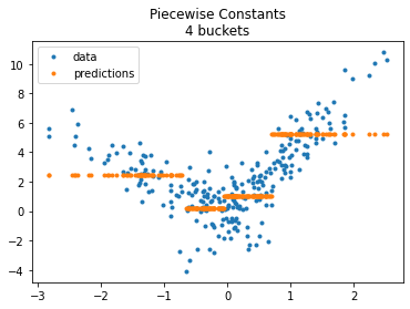
The model does not enforce continuity despite the fast it looks like so. Let’s compare with a constant on each bucket.

from sklearn.dummy import DummyRegressor
model = PiecewiseRegressor(verbose='tqdm',
                           binner=KBinsDiscretizer(n_bins=4),
                           estimator=DummyRegressor())
model.fit(X_train, y_train)

  0%|          | 0/4 [00:00<?, ?it/s][Parallel(n_jobs=1)]: Using backend SequentialBackend with 1 concurrent workers.
100%|██████████| 4/4 [00:00<?, ?it/s]
[Parallel(n_jobs=1)]: Done   4 out of   4 | elapsed:    0.0s finished

PiecewiseRegressor(binner=KBinsDiscretizer(n_bins=4),
                   estimator=DummyRegressor(), verbose='tqdm')

fig, ax = plt.subplots(1, 1)
ax.plot(X_test[:, 0], y_test, ".", label='data')
ax.plot(X_test[:, 0], model.predict(X_test), ".", label="predictions")
ax.set_title("Piecewise Constants\n4 buckets")
ax.legend();

Next

PR Model trees (M5P and co) and issue Model trees (M5P) propose an implementation a piecewise regression with any kind of regression model. It is based on Building Model Trees. It fits many models to find the best splits.