Note
Click here to download the full example code
TreeEnsembleRegressor and parallelisation#
The operator TreeEnsembleClassifier describe any tree model (decision tree, random forest, gradient boosting). The runtime is usually implements in C/C++ and uses parallelisation. The notebook studies the impact of the parallelisation.
Graph#
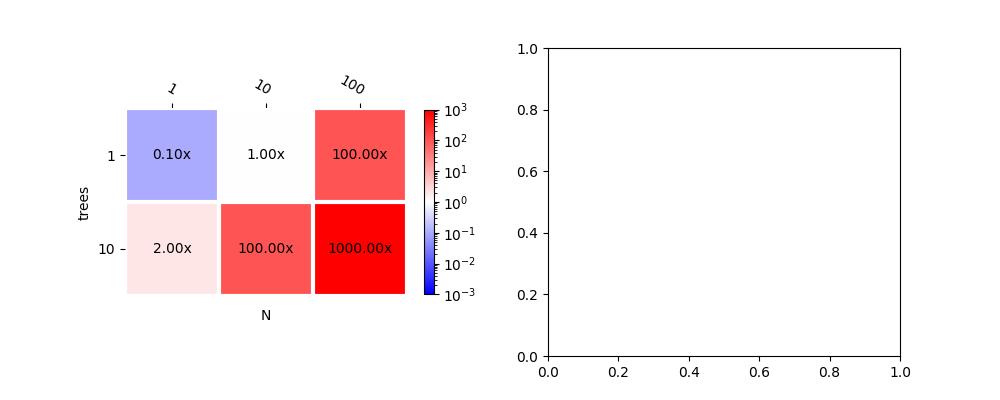
The following dummy graph shows the time ratio between two runtimes depending on the number of observations in a batch (N) and the number of trees in the forest.
from sklearn.linear_model import LogisticRegression
from sklearn.tree import DecisionTreeClassifier
from mlprodict.onnxrt import OnnxInference
from onnxruntime import InferenceSession
from skl2onnx import to_onnx
from mlprodict.onnxrt.validate.validate_benchmark import benchmark_fct
import sklearn
import numpy
from tqdm import tqdm
from sklearn.ensemble import GradientBoostingClassifier
from sklearn.datasets import make_classification
import matplotlib.pyplot as plt
from mlprodict.plotting.plotting import plot_benchmark_metrics


def plot_metric(metric, ax=None, xlabel="N", ylabel="trees", middle=1.,
                transpose=False, shrink=1.0, title=None, figsize=None):
    if figsize is not None and ax is None:
        _, ax = plt.subplots(1, 1, figsize=figsize)

    ax, cbar = plot_benchmark_metrics(
        metric, ax=ax, xlabel=xlabel, ylabel=ylabel, middle=middle,
        transpose=transpose, cbar_kw={'shrink': shrink})
    if title is not None:
        ax.set_title(title)
    return ax


data = {(1, 1): 0.1, (10, 1): 1, (1, 10): 2,
        (10, 10): 100, (100, 1): 100, (100, 10): 1000}

fig, ax = plt.subplots(1, 2, figsize=(10, 4))
plot_metric(data, ax[0], shrink=0.6)
<AxesSubplot: xlabel='N', ylabel='trees'>
plot_metric(data, ax[1], transpose=True)
<AxesSubplot: xlabel='trees', ylabel='N'>
scikit-learn: T trees vs 1 tree#
Let’s do first compare a GradientBoostingClassifier from scikit-learn with 1 tree against multiple trees.
# In[4]:


ntest = 10000
X, y = make_classification(
    n_samples=10000 + ntest, n_features=10, n_informative=5,
    n_classes=2, random_state=11)
X_train, X_test, y_train, y_test = X[:-
                                     ntest], X[-ntest:], y[:-ntest], y[-ntest:]
ModelToTest = GradientBoostingClassifier

N = [1, 10, 100, 1000, 10000]
T = [1, 2, 10, 20, 50]

models = {}
for nt in tqdm(T):
    rf = ModelToTest(n_estimators=nt, max_depth=7).fit(X_train, y_train)
    models[nt] = rf
  0%|          | 0/5 [00:00<?, ?it/s]
 20%|##        | 1/5 [00:00<00:00,  6.30it/s]
 40%|####      | 2/5 [00:00<00:00,  4.04it/s]
 60%|######    | 3/5 [00:02<00:01,  1.20it/s]
 80%|########  | 4/5 [00:05<00:01,  1.72s/it]
100%|##########| 5/5 [00:12<00:00,  3.85s/it]
100%|##########| 5/5 [00:12<00:00,  2.54s/it]
Benchmark.
def benchmark(X, fct1, fct2, N, repeat=10, number=20):

    def ti(r, n):
        if n <= 1:
            return 40 * r
        if n <= 10:
            return 10 * r
        if n <= 100:
            return 4 * r
        if n <= 1000:
            return r
        return r // 2

    with sklearn.config_context(assume_finite=True):
        # to warm up the engine
        time_kwargs = {n: dict(repeat=10, number=10) for n in N}
        benchmark_fct(fct1, X, time_kwargs=time_kwargs, skip_long_test=False)
        benchmark_fct(fct2, X, time_kwargs=time_kwargs, skip_long_test=False)
        # real measure
        time_kwargs = {n: dict(repeat=ti(repeat, n), number=number) for n in N}
        res1 = benchmark_fct(
            fct1, X, time_kwargs=time_kwargs, skip_long_test=False)
        res2 = benchmark_fct(
            fct2, X, time_kwargs=time_kwargs, skip_long_test=False)
    res = {}
    for r in sorted(res1):
        r1 = res1[r]
        r2 = res2[r]
        ratio = r2['ttime'] / r1['ttime']
        res[r] = ratio
    return res


def tree_benchmark(X, fct1, fct2, T, N, repeat=20, number=10):
    bench = {}
    for t in tqdm(T):
        if callable(X):
            x = X(t)
        else:
            x = X
        r = benchmark(x, fct1(t), fct2(t), N, repeat=repeat, number=number)
        for n, v in r.items():
            bench[n, t] = v
    return bench


bench = tree_benchmark(X_test.astype(numpy.float32),
                       lambda t: models[1].predict,
                       lambda t: models[t].predict, T, N)

list(bench.items())[:3]
  0%|          | 0/5 [00:00<?, ?it/s]
 20%|##        | 1/5 [00:15<01:00, 15.12s/it]
 40%|####      | 2/5 [00:30<00:45, 15.17s/it]
 60%|######    | 3/5 [00:46<00:31, 15.75s/it]
 80%|########  | 4/5 [01:04<00:16, 16.61s/it]
100%|##########| 5/5 [01:27<00:00, 18.73s/it]
100%|##########| 5/5 [01:27<00:00, 17.44s/it]

[((1, 1), 1.0011369814251598), ((10, 1), 0.9959889880386624), ((100, 1), 1.005397484991979)]
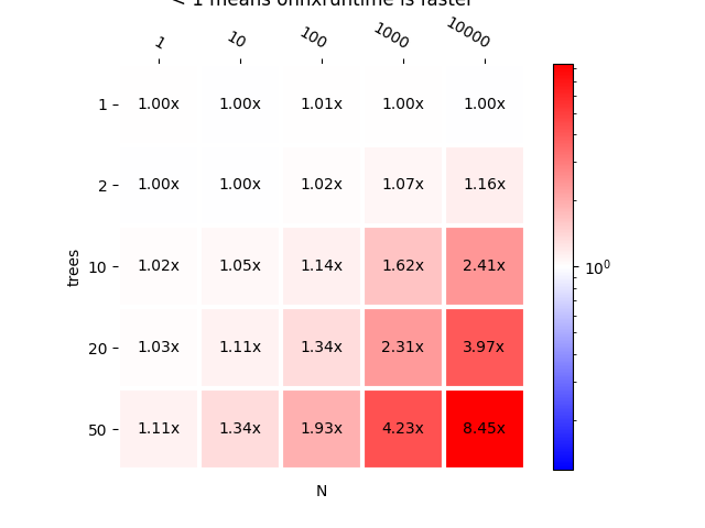
Graph.
plot_metric(bench, title="scikit-learn 1 tree vs scikit-learn T trees\n"
            "< 1 means onnxruntime is faster")
<AxesSubplot: title={'center': 'scikit-learn 1 tree vs scikit-learn T trees\n< 1 means onnxruntime is faster'}, xlabel='N', ylabel='trees'>
As expected, all ratio on first line are close to 1 since both models are the same. fourth line, second column (T=20, N=10) means an ensemble with 20 trees is slower to compute the predictions of 10 observations in a batch compare to an ensemble with 1 tree.
scikit-learn against onnxuntime#
X32 = X_test.astype(numpy.float32)
models_onnx = {t: to_onnx(m, X32[:1]) for t, m in models.items()}


sess_models = {t: InferenceSession(mo.SerializeToString())
               for t, mo in models_onnx.items()}
Benchmark.
bench_ort = tree_benchmark(
    X_test.astype(numpy.float32),
    lambda t: models[t].predict_proba,
    lambda t: (lambda x, t_=t, se=sess_models: se[t_].run(None, {'X': x})),
    T, N)
bench_ort
  0%|          | 0/5 [00:00<?, ?it/s]
 20%|##        | 1/5 [00:10<00:41, 10.38s/it]
 40%|####      | 2/5 [00:20<00:31, 10.49s/it]
 60%|######    | 3/5 [00:33<00:22, 11.47s/it]
 80%|########  | 4/5 [00:48<00:12, 12.70s/it]
100%|##########| 5/5 [01:08<00:00, 15.46s/it]
100%|##########| 5/5 [01:08<00:00, 13.70s/it]

{(1, 1): 0.10227049300818752, (10, 1): 0.11654148319861105, (100, 1): 0.2568405300796136, (1000, 1): 1.3229091818879823, (10000, 1): 3.600198469479764, (1, 2): 0.10238320664322309, (10, 2): 0.1184989188660434, (100, 2): 0.25549506446785664, (1000, 2): 1.277985529438044, (10000, 2): 3.1207165893972824, (1, 10): 0.10178234426931398, (10, 10): 0.12503913222134713, (100, 10): 0.28148667111526765, (1000, 10): 1.1409443183144472, (10000, 10): 1.8127845657152226, (1, 20): 0.10133062710596516, (10, 20): 0.13904945021252768, (100, 20): 0.25600253212772595, (1000, 20): 0.8486882067393838, (10000, 20): 1.1975173678790532, (1, 50): 0.10187102689939724, (10, 50): 0.1673120553058088, (100, 50): 0.21516157029419097, (1000, 50): 0.5869418523358603, (10000, 50): 0.7177212104403891}
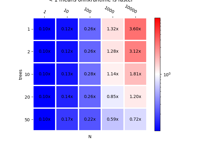
Graphs
plot_metric(bench_ort, title="scikit-learn vs onnxruntime\n < 1 "
            "means onnxruntime is faster")
<AxesSubplot: title={'center': 'scikit-learn vs onnxruntime\n < 1 means onnxruntime is faster'}, xlabel='N', ylabel='trees'>
We see onnxruntime is fast for small batches, still faster but not that much for big batches.
ZipMap operator#
ZipMap just creates a new container for the same results. The copy may impact the ratio. Let’s remove it from the equation.
X32 = X_test.astype(numpy.float32)
models_onnx = {t: to_onnx(m, X32[:1],
                          options={ModelToTest: {'zipmap': False}})
               for t, m in models.items()}

sess_models = {t: InferenceSession(mo.SerializeToString())
               for t, mo in models_onnx.items()}
Benchmarks.
bench_ort = tree_benchmark(
    X_test.astype(numpy.float32),
    lambda t: models[t].predict_proba,
    lambda t: (lambda x, t_=t, se=sess_models: se[t_].run(None, {'X': x})),
    T, N)

bench_ort
  0%|          | 0/5 [00:00<?, ?it/s]
 20%|##        | 1/5 [00:07<00:31,  7.83s/it]
 40%|####      | 2/5 [00:15<00:23,  7.93s/it]
 60%|######    | 3/5 [00:25<00:17,  8.89s/it]
 80%|########  | 4/5 [00:37<00:10, 10.08s/it]
100%|##########| 5/5 [00:55<00:00, 12.81s/it]
100%|##########| 5/5 [00:55<00:00, 11.09s/it]

{(1, 1): 0.08798600208974772, (10, 1): 0.0911144626980488, (100, 1): 0.10383884774190465, (1000, 1): 0.1273027292314435, (10000, 1): 0.1938153993389047, (1, 2): 0.08794266846621691, (10, 2): 0.0927500404876507, (100, 2): 0.10635945366629987, (1000, 2): 0.13748626005844075, (10000, 2): 0.1997658866658732, (1, 10): 0.08831790632307972, (10, 10): 0.10184311942454842, (100, 10): 0.15272700247842572, (1000, 10): 0.3265126290803524, (10000, 10): 0.4877729136908548, (1, 20): 0.08917151013876999, (10, 20): 0.11661491837577477, (100, 20): 0.14548205627568078, (1000, 20): 0.28771134247360586, (10000, 20): 0.402481379883806, (1, 50): 0.09071633578778325, (10, 50): 0.15346270146857977, (100, 50): 0.14558536813255007, (1000, 50): 0.2776309990033727, (10000, 50): 0.3438503669422623}
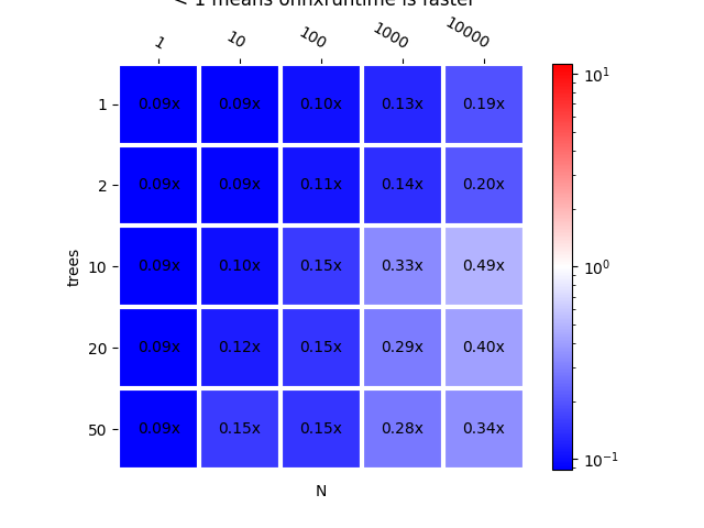
Graphs.
plot_metric(bench_ort, title="scikit-learn vs onnxruntime (no zipmap)\n < 1 "
            "means onnxruntime is faster")


# ZipMap removal significantly improves.
#
# Implementation details for mlprodict runtime
# ++++++++++++++++++++++++++++++++++++++++++++
#
# The runtime implemented in :epkg:`mlprodict` mostly relies on
# two files:
# * `op_tree_ensemble_common_p_agg_.hpp <https://github.com/sdpython/
#   mlprodict/blob/master/mlprodict/onnxrt/ops_cpu/
#   op_tree_ensemble_common_p_agg_.hpp>`_
# * `op_tree_ensemble_common_p_.hpp <https://github.com/sdpython/
#   mlprodict/blob/master/mlprodict/onnxrt/ops_cpu/
#   op_tree_ensemble_common_p_.hpp>`_
#
# The runtime builds a tree structure, computes the output of every
# tree and then agregates them. The implementation distringuishes
# when the batch size contains only 1 observations or many.
# It parallelizes on the following conditions:
# * if the batch size $N \geqslant N_0$, it then parallelizes per
#   observation, asuming every one is independant,
# * if the batch size $N = 1$ and the number of trees
#   $T \geqslant T_0$, it then parallelizes per tree.
#
# scikit-learn against mlprodict, no parallelisation
# ++++++++++++++++++++++++++++++++++++++++++++++++++


oinf_models = {t: OnnxInference(mo, runtime="python_compiled")
               for t, mo in models_onnx.items()}
Let’s modify the thresholds which trigger the parallelization.
for _, oinf in oinf_models.items():
    oinf.sequence_[0].ops_.rt_.omp_tree_ = 10000000
    oinf.sequence_[0].ops_.rt_.omp_N_ = 10000000
Benchmarks.
bench_mlp = tree_benchmark(
    X_test.astype(numpy.float32),
    lambda t: models[t].predict,
    lambda t: (lambda x, t_=t, oi=oinf_models: oi[t_].run({'X': x})),
    T, N)
bench_mlp
  0%|          | 0/5 [00:00<?, ?it/s]
 20%|##        | 1/5 [00:08<00:33,  8.37s/it]
 40%|####      | 2/5 [00:17<00:25,  8.55s/it]
 60%|######    | 3/5 [00:29<00:20, 10.23s/it]
 80%|########  | 4/5 [00:46<00:13, 13.15s/it]
100%|##########| 5/5 [01:19<00:00, 20.24s/it]
100%|##########| 5/5 [01:19<00:00, 15.94s/it]

{(1, 1): 0.05250026671226264, (10, 1): 0.055318610818540746, (100, 1): 0.07986082578132989, (1000, 1): 0.2453230276458112, (10000, 1): 0.5618135619311029, (1, 2): 0.052766554267586606, (10, 2): 0.05744266757316101, (100, 2): 0.0932531949491305, (1000, 2): 0.3225047095569382, (10000, 2): 0.7092584023279892, (1, 10): 0.053871616832349735, (10, 10): 0.07090374073337581, (100, 10): 0.21371074087308423, (1000, 10): 0.8575582917741711, (10000, 10): 1.4851486945730787, (1, 20): 0.05526400590413813, (10, 20): 0.09169793185582159, (100, 20): 0.3740256322541707, (1000, 20): 1.3710143309041296, (10000, 20): 2.0814724037824113, (1, 50): 0.059598627829410555, (10, 50): 0.13079132586651543, (100, 50): 0.6364370047354984, (1000, 50): 1.9008988567112426, (10000, 50): 2.484952490169669}
Graphs.
plot_metric(bench_mlp, title="scikit-learn vs mlprodict\n < 1 "
            "means mlprodict is faster")
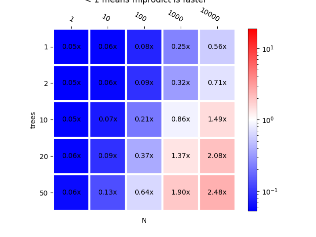
<AxesSubplot: title={'center': 'scikit-learn vs mlprodict\n < 1 means mlprodict is faster'}, xlabel='N', ylabel='trees'>
Let’s compare onnxruntime against mlprodict.
bench_mlp_ort = tree_benchmark(
    X_test.astype(numpy.float32),
    lambda t: (lambda x, t_=t, se=sess_models: se[t_].run(None, {'X': x})),
    lambda t: (lambda x, t_=t, oi=oinf_models: oi[t_].run({'X': x})),
    T, N)
bench_mlp_ort
  0%|          | 0/5 [00:00<?, ?it/s]
 20%|##        | 1/5 [00:01<00:06,  1.56s/it]
 40%|####      | 2/5 [00:03<00:05,  1.71s/it]
 60%|######    | 3/5 [00:08<00:06,  3.18s/it]
 80%|########  | 4/5 [00:17<00:05,  5.58s/it]
100%|##########| 5/5 [00:38<00:00, 11.13s/it]
100%|##########| 5/5 [00:38<00:00,  7.71s/it]

{(1, 1): 0.6323186276590774, (10, 1): 0.6439543687434605, (100, 1): 0.8139814863871733, (1000, 1): 2.0454252155446806, (10000, 1): 3.3828064278005265, (1, 2): 0.6327250531950117, (10, 2): 0.6487772751330764, (100, 2): 0.9285250297914696, (1000, 2): 2.475833602034365, (10000, 2): 3.696624711985688, (1, 10): 0.642662695873458, (10, 10): 0.7285538182910188, (100, 10): 1.281688752089102, (1000, 10): 2.727234466872367, (10000, 10): 3.1368189381196077, (1, 20): 0.6565574413854028, (10, 20): 0.8250422682240249, (100, 20): 2.7480248382948305, (1000, 20): 4.9604829921593225, (10000, 20): 5.293900246781706, (1, 50): 0.6927219136494578, (10, 50): 0.8933321679883014, (100, 50): 4.505604756258499, (1000, 50): 6.955433343487955, (10000, 50): 7.2505487290375665}
Graphs.
plot_metric(bench_mlp_ort, title="onnxruntime vs mlprodict\n < 1 means "
            "mlprodict is faster\nno parallelisation")
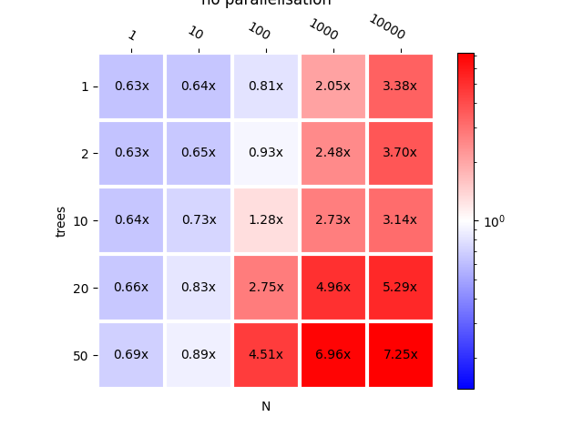
<AxesSubplot: title={'center': 'onnxruntime vs mlprodict\n < 1 means mlprodict is faster\nno parallelisation'}, xlabel='N', ylabel='trees'>
This implementation is faster except for high number of trees or high number of observations. Let’s add parallelisation for trees and observations.
for _, oinf in oinf_models.items():
    oinf.sequence_[0].ops_.rt_.omp_tree_ = 2
    oinf.sequence_[0].ops_.rt_.omp_N_ = 2


bench_mlp_para = tree_benchmark(
    X_test.astype(numpy.float32),
    lambda t: models[t].predict,
    lambda t: (lambda x, t_=t, oi=oinf_models: oi[t_].run({'X': x})),
    T, N)

bench_mlp_para
  0%|          | 0/5 [00:00<?, ?it/s]
 20%|##        | 1/5 [00:23<01:35, 23.99s/it]
 40%|####      | 2/5 [00:44<01:05, 21.81s/it]
 60%|######    | 3/5 [01:32<01:08, 34.08s/it]
 80%|########  | 4/5 [02:52<00:51, 51.84s/it]
100%|##########| 5/5 [03:54<00:00, 55.52s/it]
100%|##########| 5/5 [03:54<00:00, 46.81s/it]

{(1, 1): 0.05205642664675265, (10, 1): 8.232928662090673, (100, 1): 3.8397530874864847, (1000, 1): 7.032643064375739, (10000, 1): 2.1197485060434733, (1, 2): 0.05228053963375641, (10, 2): 4.740109809546292, (100, 2): 4.8630437402757805, (1000, 2): 6.643634784959738, (10000, 2): 1.9763541473935924, (1, 10): 4.552766536704755, (10, 10): 6.2110982823242455, (100, 10): 4.328893997195667, (1000, 10): 5.7009128789780465, (10000, 10): 1.5622270919697556, (1, 20): 9.07437715116346, (10, 20): 9.629977615474784, (100, 20): 8.232514738791371, (1000, 20): 4.6963671868293035, (10000, 20): 1.1649030536356886, (1, 50): 5.583120541323525, (10, 50): 3.581654543892374, (100, 50): 3.8950247270178413, (1000, 50): 2.6650878385369023, (10000, 50): 0.7152097824872292}
Graphs.
plot_metric(bench_mlp_para, title="scikit-learn vs mlprodict\n < 1 means "
            "mlprodict is faster\nparallelisation")
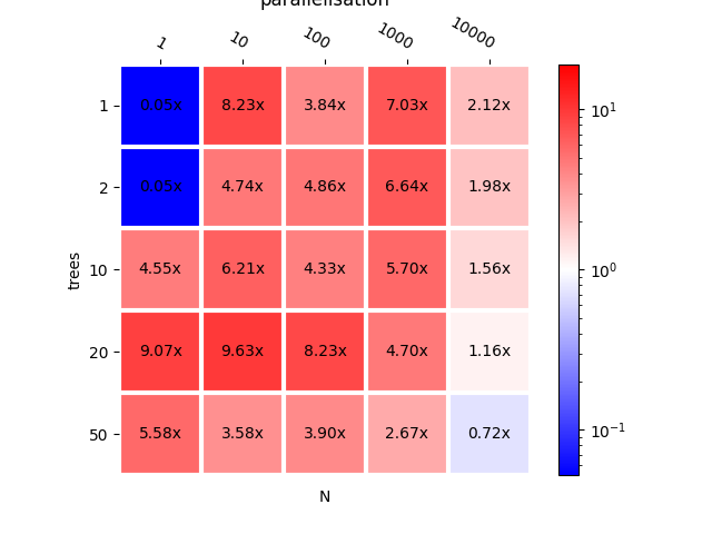
<AxesSubplot: title={'center': 'scikit-learn vs mlprodict\n < 1 means mlprodict is faster\nparallelisation'}, xlabel='N', ylabel='trees'>
Parallelisation does improve the computation time when N is big. Let’s compare with and without parallelisation.
bench_para = {}
for k, v in bench_mlp.items():
    bench_para[k] = bench_mlp_para[k] / v


plot_metric(bench_para, title="mlprodict vs mlprodict parallelized\n < 1 "
            "means parallelisation is faster")
<AxesSubplot: title={'center': 'mlprodict vs mlprodict parallelized\n < 1 means parallelisation is faster'}, xlabel='N', ylabel='trees'>
Parallelisation per trees does not seem to be efficient. Let’s confirm with a proper benchmark as the previous merges results from two benchmarks.
for _, oinf in oinf_models.items():
    oinf.sequence_[0].ops_.rt_.omp_tree_ = 1000000
    oinf.sequence_[0].ops_.rt_.omp_N_ = 1000000

oinf_models_para = {t: OnnxInference(mo, runtime="python_compiled")
                    for t, mo in models_onnx.items()}

for _, oinf in oinf_models_para.items():
    oinf.sequence_[0].ops_.rt_.omp_tree_ = 2
    oinf.sequence_[0].ops_.rt_.omp_N_ = 2

bench_mlp_para = tree_benchmark(
    X_test.astype(numpy.float32),
    lambda t: (lambda x, t_=t, oi=oinf_models: oi[t_].run({'X': x})),
    lambda t: (lambda x, t_=t, oi=oinf_models_para: oi[t_].run({'X': x})),
    T, N, repeat=20, number=20)

bench_mlp_para
  0%|          | 0/5 [00:00<?, ?it/s]
 20%|##        | 1/5 [00:25<01:40, 25.02s/it]
 40%|####      | 2/5 [00:48<01:11, 23.87s/it]
 60%|######    | 3/5 [02:44<02:12, 66.32s/it]
 80%|########  | 4/5 [04:29<01:21, 81.27s/it]
100%|##########| 5/5 [06:51<00:00, 103.47s/it]
100%|##########| 5/5 [06:51<00:00, 82.39s/it]

{(1, 1): 0.9948310142913012, (10, 1): 62.90692250302435, (100, 1): 117.50392909857285, (1000, 1): 18.681690442434622, (10000, 1): 3.542811026404204, (1, 2): 0.9996758959286081, (10, 2): 73.67589193923493, (100, 2): 47.683365742281815, (1000, 2): 18.45452465367828, (10000, 2): 2.6639991514970944, (1, 10): 151.4670710876751, (10, 10): 117.64229613605362, (100, 10): 17.57888344088909, (1000, 10): 5.01330258430993, (10000, 10): 1.0626741882464912, (1, 20): 110.28441066038202, (10, 20): 66.48248925473392, (100, 20): 14.945074149775296, (1000, 20): 4.06758543410752, (10000, 20): 0.5673688333712591, (1, 50): 115.99694973738409, (10, 50): 53.725383414325364, (100, 50): 7.03009446831395, (1000, 50): 1.445527287508299, (10000, 50): 0.29507962290260026}
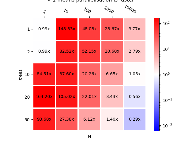
Graph.
plot_metric(bench_mlp_para, title="mlprodict vs mlprodict parallelized\n < 1 "
            "means parallelisation is faster\nsame baseline")
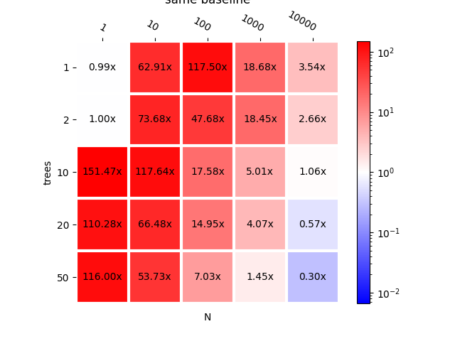
<AxesSubplot: title={'center': 'mlprodict vs mlprodict parallelized\n < 1 means parallelisation is faster\nsame baseline'}, xlabel='N', ylabel='trees'>
It should be run on different machines. On the current one, parallelisation per trees (when N=1) does not seem to help. Parallelisation for a small number of observations does not seem to help either. So we need to find some threshold.
Parallelisation per trees#
Let’s study the parallelisation per tree. We need to train new models.
# In[33]:


N2 = [1, 10]
T2 = [1, 2, 10, 50, 100, 150, 200, 300, 400, 500]

models2 = {}
for nt in tqdm(T2):
    rf = ModelToTest(n_estimators=nt, max_depth=7).fit(X_train, y_train)
    models2[nt] = rf
  0%|          | 0/10 [00:00<?, ?it/s]
 10%|#         | 1/10 [00:00<00:01,  6.38it/s]
 20%|##        | 2/10 [00:00<00:01,  4.05it/s]
 30%|###       | 3/10 [00:02<00:05,  1.20it/s]
 40%|####      | 4/10 [00:09<00:21,  3.52s/it]
 50%|#####     | 5/10 [00:24<00:38,  7.74s/it]
 60%|######    | 6/10 [00:47<00:51, 12.87s/it]
 70%|#######   | 7/10 [01:18<00:55, 18.58s/it]
 80%|########  | 8/10 [02:03<00:54, 27.15s/it]
 90%|######### | 9/10 [03:04<00:37, 37.74s/it]
100%|##########| 10/10 [04:21<00:00, 49.71s/it]
100%|##########| 10/10 [04:21<00:00, 26.11s/it]
Conversion to ONNX.
X32 = X_test.astype(numpy.float32)
models2_onnx = {t: to_onnx(m, X32[:1]) for t, m in models2.items()}

oinf_models2 = {t: OnnxInference(mo, runtime="python_compiled")
                for t, mo in models2_onnx.items()}
for _, oinf in oinf_models2.items():
    oinf.sequence_[0].ops_.rt_.omp_tree_ = 1000000
    oinf.sequence_[0].ops_.rt_.omp_N_ = 1000000

oinf_models2_para = {t: OnnxInference(
    mo, runtime="python_compiled") for t, mo in models2_onnx.items()}
for _, oinf in oinf_models2_para.items():
    oinf.sequence_[0].ops_.rt_.omp_tree_ = 2
    oinf.sequence_[0].ops_.rt_.omp_N_ = 100
And benchmark.
# In[36]:


bench_mlp_tree = tree_benchmark(
    X_test.astype(numpy.float32),
    lambda t: (lambda x, t_=t, oi=oinf_models2: oi[t_].run({'X': x})),
    lambda t: (lambda x, t_=t, oi=oinf_models2_para: oi[t_].run({'X': x})),
    T2, N2, repeat=20, number=20)
bench_mlp_tree
  0%|          | 0/10 [00:00<?, ?it/s]
 10%|#         | 1/10 [00:01<00:16,  1.89s/it]
 20%|##        | 2/10 [00:03<00:15,  1.90s/it]
 30%|###       | 3/10 [00:42<02:09, 18.55s/it]
 40%|####      | 4/10 [01:23<02:44, 27.46s/it]
 50%|#####     | 5/10 [02:13<02:58, 35.60s/it]
 60%|######    | 6/10 [03:08<02:48, 42.21s/it]
 70%|#######   | 7/10 [04:03<02:19, 46.47s/it]
 80%|########  | 8/10 [05:16<01:49, 54.78s/it]
 90%|######### | 9/10 [08:03<01:30, 90.02s/it]
100%|##########| 10/10 [11:07<00:00, 118.90s/it]
100%|##########| 10/10 [11:07<00:00, 66.72s/it]

{(1, 1): 1.0008572795574162, (10, 1): 0.998439986975673, (1, 2): 1.002155326796771, (10, 2): 1.001684660958159, (1, 10): 31.444042682330767, (10, 10): 58.60594365578326, (1, 50): 40.29122693202075, (10, 50): 10.695505471938697, (1, 100): 32.43367012348174, (10, 100): 21.25979785856979, (1, 150): 34.510245096262956, (10, 150): 8.724880543811897, (1, 200): 33.33046864361148, (10, 200): 4.988662143673411, (1, 300): 14.641392427233432, (10, 300): 5.593011810245873, (1, 400): 23.522461622383734, (10, 400): 3.0734608590786414, (1, 500): 15.827910785537107, (10, 500): 3.044979714783015}
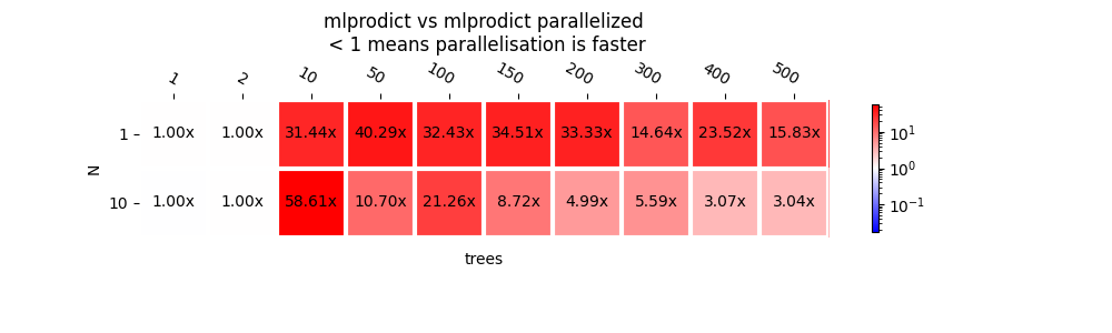
Graph.
plot_metric(
    bench_mlp_tree, transpose=True, figsize=(10, 3), shrink=0.5,
    title="mlprodict vs mlprodict parallelized\n < 1 means parallelisation "
    "is faster")
<AxesSubplot: title={'center': 'mlprodict vs mlprodict parallelized\n < 1 means parallelisation is faster'}, xlabel='trees', ylabel='N'>
The parallelisation starts to be below 1 after 400 trees. For 10 observations, there is no parallelisation neither by trees nor by observations. Ratios are close to 1. The gain obviously depends on the tree depth. You can try with a different max depth and the number of trees parallelisation becomes interesting depending on the tree depth.
Multi-Class DecisionTreeClassifier#
Same experiment when the number of tree is 1 but then we change the number of classes.
ModelToTest = DecisionTreeClassifier

C = [2, 5, 10, 15, 20, 30, 40, 50]
N = [1, 10, 100, 1000, 10000]
trees = {}
for cl in tqdm(C):

    ntest = 10000
    X, y = make_classification(
        n_samples=10000 + ntest, n_features=12, n_informative=8,
        n_classes=cl, random_state=11)
    X_train, X_test, y_train, y_test = (
        X[:-ntest], X[-ntest:], y[:-ntest], y[-ntest:])

    dt = ModelToTest(max_depth=7).fit(X_train, y_train)

    X32 = X_test.astype(numpy.float32)
    monnx = to_onnx(dt, X32[:1])
    oinf = OnnxInference(monnx)
    oinf.sequence_[0].ops_.rt_.omp_N_ = 1000000
    trees[cl] = dict(model=dt, X_test=X_test, X32=X32, monnx=monnx, oinf=oinf)


bench_dt = tree_benchmark(lambda cl: trees[cl]['X32'],
                          lambda cl: trees[cl]['model'].predict_proba,
                          lambda cl: (
                              lambda x, c=cl: trees[c]['oinf'].run({'X': x})),
                          C, N)

bench_dt
  0%|          | 0/8 [00:00<?, ?it/s]
 12%|#2        | 1/8 [00:00<00:01,  3.51it/s]
 25%|##5       | 2/8 [00:00<00:01,  3.37it/s]
 38%|###7      | 3/8 [00:00<00:01,  3.16it/s]
 50%|#####     | 4/8 [00:01<00:01,  2.94it/s]
 62%|######2   | 5/8 [00:01<00:01,  2.75it/s]
 75%|#######5  | 6/8 [00:02<00:00,  2.47it/s]
 88%|########7 | 7/8 [00:02<00:00,  2.22it/s]
100%|##########| 8/8 [00:03<00:00,  2.00it/s]
100%|##########| 8/8 [00:03<00:00,  2.39it/s]

  0%|          | 0/8 [00:00<?, ?it/s]
 12%|#2        | 1/8 [00:04<00:30,  4.39s/it]
 25%|##5       | 2/8 [00:09<00:27,  4.54s/it]
 38%|###7      | 3/8 [00:14<00:23,  4.76s/it]
 50%|#####     | 4/8 [00:19<00:19,  4.99s/it]
 62%|######2   | 5/8 [00:25<00:15,  5.23s/it]
 75%|#######5  | 6/8 [00:31<00:11,  5.55s/it]
 88%|########7 | 7/8 [00:37<00:05,  5.94s/it]
100%|##########| 8/8 [00:45<00:00,  6.37s/it]
100%|##########| 8/8 [00:45<00:00,  5.66s/it]

{(1, 2): 0.5144306219894155, (10, 2): 0.497636512336468, (100, 2): 0.5164181839225809, (1000, 2): 0.6533015164762946, (10000, 2): 0.8495108081323643, (1, 5): 0.5001570414753025, (10, 5): 0.49875105359046096, (100, 5): 0.5331060959512705, (1000, 5): 0.6888425501120783, (10000, 5): 0.8682387231720484, (1, 10): 0.49898086418921705, (10, 10): 0.49889734939049735, (100, 10): 0.5290783649263836, (1000, 10): 0.6581123466964187, (10000, 10): 0.8054445837702259, (1, 15): 0.4974556258496031, (10, 15): 0.4915023500586425, (100, 15): 0.5249748092476151, (1000, 15): 0.6511301201020304, (10000, 15): 0.7894947340668653, (1, 20): 0.5098614980581243, (10, 20): 0.4907603987291428, (100, 20): 0.526560101373793, (1000, 20): 0.6342275234590019, (10000, 20): 0.7529344971881822, (1, 30): 0.49585466269599127, (10, 30): 0.5016835876359774, (100, 30): 0.5385027735100477, (1000, 30): 0.6108189633365876, (10000, 30): 0.7209619832961572, (1, 40): 0.5004123038615591, (10, 40): 0.5027519733799634, (100, 40): 0.5337144755215893, (1000, 40): 0.6051860178909579, (10000, 40): 0.7271436179118411, (1, 50): 0.5001655880183867, (10, 50): 0.5073789721289271, (100, 50): 0.5527602294063638, (1000, 50): 0.6072395741192154, (10000, 50): 0.7286257886115594}
Graph.
plot_metric(bench_dt, ylabel="classes", transpose=True, shrink=0.75,
            title="scikit-learn vs mlprodict (DecisionTreeClassifier) \n"
            "< 1 means mlprodict is faster\n no parallelisation")
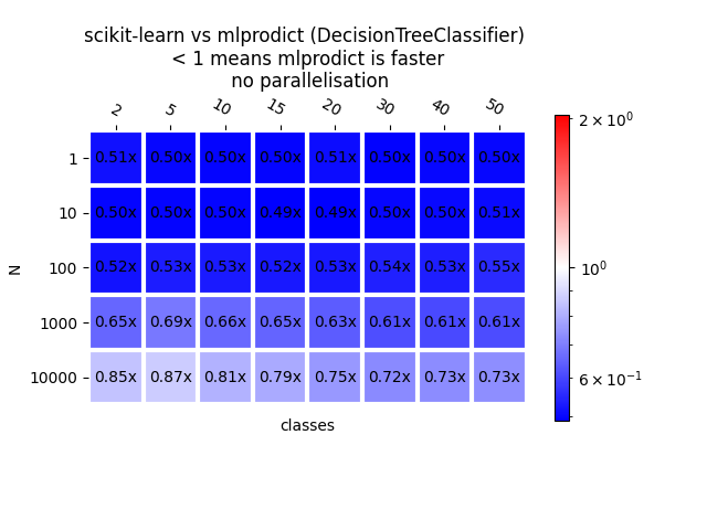
<AxesSubplot: title={'center': 'scikit-learn vs mlprodict (DecisionTreeClassifier) \n< 1 means mlprodict is faster\n no parallelisation'}, xlabel='classes', ylabel='N'>
Multi-class LogisticRegression#
ModelToTest = LogisticRegression

C = [2, 5, 10, 15, 20]
N = [1, 10, 100, 1000, 10000]

models = {}
for cl in tqdm(C):

    ntest = 10000
    X, y = make_classification(
        n_samples=10000 + ntest, n_features=10, n_informative=6,
        n_classes=cl, random_state=11)
    X_train, X_test, y_train, y_test = (
        X[:-ntest], X[-ntest:], y[:-ntest], y[-ntest:])

    model = ModelToTest().fit(X_train, y_train)

    X32 = X_test.astype(numpy.float32)
    monnx = to_onnx(model, X32[:1])
    oinf = OnnxInference(monnx)
    models[cl] = dict(model=model, X_test=X_test,
                      X32=X32, monnx=monnx, oinf=oinf)


bench_lr = tree_benchmark(lambda cl: models[cl]['X32'],
                          lambda cl: models[cl]['model'].predict_proba,
                          lambda cl: (
                              lambda x, c=cl: trees[c]['oinf'].run({'X': x})),
                          C, N)
bench_lr
  0%|          | 0/5 [00:00<?, ?it/s]
 20%|##        | 1/5 [00:00<00:00,  7.22it/s]
 40%|####      | 2/5 [00:00<00:00,  3.20it/s]
 60%|######    | 3/5 [00:00<00:00,  2.88it/s]
 80%|########  | 4/5 [00:01<00:00,  2.07it/s]
100%|##########| 5/5 [00:02<00:00,  1.66it/s]
100%|##########| 5/5 [00:02<00:00,  2.02it/s]

  0%|          | 0/5 [00:00<?, ?it/s]
 20%|##        | 1/5 [00:05<00:20,  5.03s/it]
 40%|####      | 2/5 [00:12<00:18,  6.27s/it]
 60%|######    | 3/5 [00:20<00:14,  7.28s/it]
 80%|########  | 4/5 [00:30<00:08,  8.14s/it]
100%|##########| 5/5 [00:40<00:00,  9.05s/it]
100%|##########| 5/5 [00:40<00:00,  8.16s/it]

{(1, 2): 0.3822994099338818, (10, 2): 0.3937276804869186, (100, 2): 0.42612909112528136, (1000, 2): 0.5816026186134228, (10000, 2): 1.0284729494869294, (1, 5): 0.3105780013038795, (10, 5): 0.29999681308336235, (100, 5): 0.3040375938205441, (1000, 5): 0.308188609724216, (10000, 5): 0.3296122193658053, (1, 10): 0.3022993841090566, (10, 10): 0.2761580338886293, (100, 10): 0.2870191834890792, (1000, 10): 0.2545346224521646, (10000, 10): 0.23363557506168794, (1, 15): 0.3088835319714267, (10, 15): 0.29170438338467913, (100, 15): 0.2745552095213862, (1000, 15): 0.22748019331334057, (10000, 15): 0.2090149176832754, (1, 20): 0.31211271884795466, (10, 20): 0.2889349967122497, (100, 20): 0.2594277673369473, (1000, 20): 0.2006647064726369, (10000, 20): 0.18831338050247373}
Graph.
plot_metric(bench_lr, ylabel="classes",
            title="scikit-learn vs mlprodict (LogisticRegression) \n"
            "< 1 means mlprodict is faster\n no parallelisation")
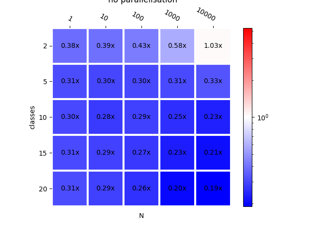
<AxesSubplot: title={'center': 'scikit-learn vs mlprodict (LogisticRegression) \n< 1 means mlprodict is faster\n no parallelisation'}, xlabel='N', ylabel='classes'>
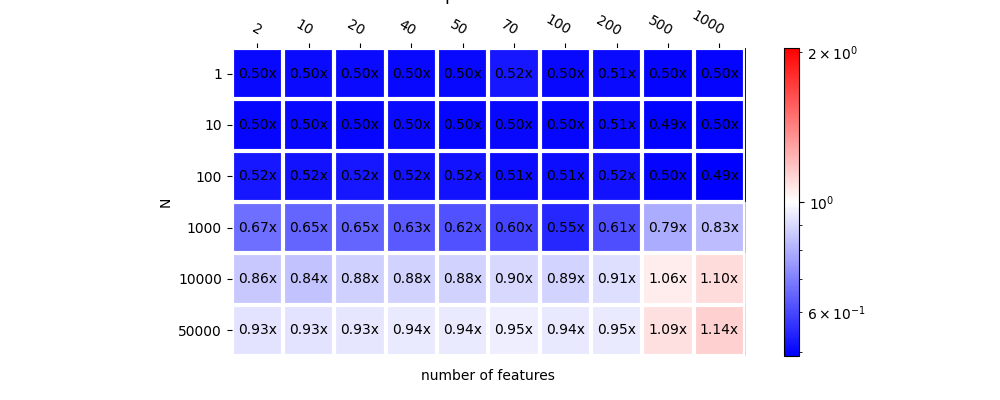
Decision Tree and number of features#
ModelToTest = DecisionTreeClassifier

NF = [2, 10, 20, 40, 50, 70, 100, 200, 500, 1000]
N = [1, 10, 100, 1000, 10000, 50000]
trees_nf = {}

for nf in tqdm(NF):
    ntest = 10000
    X, y = make_classification(
        n_samples=10000 + ntest, n_features=nf, n_informative=nf // 2 + 1,
        n_redundant=0, n_repeated=0,
        n_classes=2, random_state=11)
    X_train, X_test, y_train, y_test = (
        X[:-ntest], X[-ntest:], y[:-ntest], y[-ntest:])

    dt = ModelToTest(max_depth=7).fit(X_train, y_train)

    X32 = X_test.astype(numpy.float32)
    monnx = to_onnx(dt, X32[:1])
    oinf = OnnxInference(monnx)
    oinf.sequence_[0].ops_.rt_.omp_N_ = 1000000
    trees_nf[nf] = dict(model=dt, X_test=X_test,
                        X32=X32, monnx=monnx, oinf=oinf)


bench_dt_nf = tree_benchmark(
    lambda nf: trees_nf[nf]['X32'],
    lambda nf: trees_nf[nf]['model'].predict_proba,
    lambda nf: (lambda x, c=nf: trees_nf[c]['oinf'].run({'X': x})), NF, N)
bench_dt_nf
  0%|          | 0/10 [00:00<?, ?it/s]
 20%|##        | 2/10 [00:00<00:01,  5.81it/s]
 30%|###       | 3/10 [00:00<00:01,  3.53it/s]
 40%|####      | 4/10 [00:01<00:02,  2.05it/s]
 50%|#####     | 5/10 [00:02<00:03,  1.48it/s]
 60%|######    | 6/10 [00:04<00:03,  1.09it/s]
 70%|#######   | 7/10 [00:06<00:03,  1.28s/it]
 80%|########  | 8/10 [00:10<00:04,  2.14s/it]
 90%|######### | 9/10 [00:20<00:04,  4.65s/it]
100%|##########| 10/10 [00:41<00:00,  9.69s/it]
100%|##########| 10/10 [00:41<00:00,  4.14s/it]

  0%|          | 0/10 [00:00<?, ?it/s]
 10%|#         | 1/10 [00:07<01:06,  7.38s/it]
 20%|##        | 2/10 [00:14<00:59,  7.42s/it]
 30%|###       | 3/10 [00:22<00:52,  7.54s/it]
 40%|####      | 4/10 [00:30<00:46,  7.67s/it]
 50%|#####     | 5/10 [00:38<00:38,  7.76s/it]
 60%|######    | 6/10 [00:46<00:31,  7.88s/it]
 70%|#######   | 7/10 [00:54<00:24,  8.08s/it]
 80%|########  | 8/10 [01:05<00:17,  8.91s/it]
 90%|######### | 9/10 [01:21<00:10, 10.94s/it]
100%|##########| 10/10 [01:38<00:00, 12.85s/it]
100%|##########| 10/10 [01:38<00:00,  9.81s/it]

{(1, 2): 0.5017787585285354, (10, 2): 0.4984701412893032, (100, 2): 0.5214294369312159, (1000, 2): 0.6663441727104532, (10000, 2): 0.859443810824273, (50000, 2): 0.9254061953458351, (1, 10): 0.504881777217451, (10, 10): 0.5023072615452562, (100, 10): 0.5165548560760278, (1000, 10): 0.6484845268066077, (10000, 10): 0.843363264706442, (50000, 10): 0.9263579434938217, (1, 20): 0.5045857187521313, (10, 20): 0.5011843056089655, (100, 20): 0.5211572841013247, (1000, 20): 0.6500112244529652, (10000, 20): 0.8778600280718336, (50000, 20): 0.9345597527663726, (1, 40): 0.5035081952032284, (10, 40): 0.5041440062039214, (100, 40): 0.5161873460795032, (1000, 40): 0.631239112230863, (10000, 40): 0.8831667952875879, (50000, 40): 0.9434640122873941, (1, 50): 0.5026044157831395, (10, 50): 0.5002446789520113, (100, 50): 0.5173798734946722, (1000, 50): 0.6163194221815674, (10000, 50): 0.8828360279547315, (50000, 50): 0.9448076949107291, (1, 70): 0.5217896491793713, (10, 70): 0.5020516956805138, (100, 70): 0.5088439794116499, (1000, 70): 0.5950264493991858, (10000, 70): 0.8961835227250717, (50000, 70): 0.9532483885197998, (1, 100): 0.5019378493439284, (10, 100): 0.5006571034870443, (100, 100): 0.5078691278688382, (1000, 100): 0.5463778588695178, (10000, 100): 0.8863256067537802, (50000, 100): 0.9368169517139237, (1, 200): 0.505353618934832, (10, 200): 0.5059105731091714, (100, 200): 0.5160628300207575, (1000, 200): 0.6113203492083846, (10000, 200): 0.9146306662474537, (50000, 200): 0.9452543592878064, (1, 500): 0.49775754224314295, (10, 500): 0.4949786400879252, (100, 500): 0.49824890658273396, (1000, 500): 0.7943423644391288, (10000, 500): 1.0557019796338265, (50000, 500): 1.0903854694561212, (1, 1000): 0.49672279760332294, (10, 1000): 0.49507510517946096, (100, 1000): 0.4901766095354515, (1000, 1000): 0.8279650923759263, (10000, 1000): 1.1029929526653837, (50000, 1000): 1.140427353760382}
Graph.
plot_metric(
    bench_dt_nf, ylabel="number of features", transpose=True, figsize=(10, 4),
    title="scikit-learn vs mlprodict (DecisionTreeClassifier) \n"
    "< 1 means mlprodict is faster\n no parallelisation")
<AxesSubplot: title={'center': 'scikit-learn vs mlprodict (DecisionTreeClassifier) \n< 1 means mlprodict is faster\n no parallelisation'}, xlabel='number of features', ylabel='N'>
Total running time of the script: ( 36 minutes 33.124 seconds)