Fast TopK elements

Links: notebook, html, PDF, python, slides, GitHub

Looking for the top k elements is something needed to implement a simple k nearest neighbors. The implementation scikit-learn is using relies on numpy: _kneighbors_reduce_func. mlprodict also contains a C++ implementation of the same function. Let’s compare them.

from jyquickhelper import add_notebook_menu
add_notebook_menu()

%matplotlib inline

Two implementations

We assume we are looking for the k nearest elements of every row of matrix X which is a dense matrix of doubles.

import numpy.random as rnd
from sklearn.neighbors._base import KNeighborsMixin

mixin = KNeighborsMixin()

def topk_sklearn(X, k):
    return mixin._kneighbors_reduce_func(X, 0, k, False)

X = rnd.randn(5, 10)
ind = topk_sklearn(X, 3)
ind

array([[2, 7, 3],
       [7, 0, 8],
       [1, 5, 6],
       [8, 9, 3],
       [4, 6, 5]], dtype=int64)

Now the implementation with mlprodict (C++) available at topk_element_min. It uses heap.

from mlprodict.onnxrt.ops_cpu._op_onnx_numpy import topk_element_min_double

def topk_cpp(X, k):
    return topk_element_min_double(X, k, True, 50)

ind = topk_cpp(X, 3)
ind

array([[2, 7, 3],
       [7, 0, 8],
       [1, 5, 6],
       [8, 9, 3],
       [4, 6, 5]], dtype=int64)

Speed comparison by size

%timeit topk_sklearn(X, 3)

21.7 µs ± 4.19 µs per loop (mean ± std. dev. of 7 runs, 100000 loops each)

%timeit topk_cpp(X, 3)

4.1 µs ± 435 ns per loop (mean ± std. dev. of 7 runs, 100000 loops each)

Quite a lot faster on this simple example. Let’s look for bigger matrices.

X = rnd.randn(1000, 100)

%timeit topk_sklearn(X, 10)

1.8 ms ± 102 µs per loop (mean ± std. dev. of 7 runs, 1000 loops each)

%timeit topk_cpp(X, 10)

786 µs ± 116 µs per loop (mean ± std. dev. of 7 runs, 1000 loops each)

from cpyquickhelper.numbers import measure_time
from tqdm import tqdm
from pandas import DataFrame

rows = []
for n in tqdm(range(1000, 10001, 1000)):
    X = rnd.randn(n, 1000)
    res = measure_time('topk_sklearn(X, 20)',
                       {'X': X, 'topk_sklearn': topk_sklearn},
                       div_by_number=True,
                       number=2, repeat=2)
    res["N"] = n
    res["name"] = 'topk_sklearn'
    rows.append(res)
    res = measure_time('topk_cpp(X, 20)',
                       {'X': X, 'topk_cpp': topk_cpp},
                       div_by_number=True,
                       number=4, repeat=4)
    res["N"] = n
    res["name"] = 'topk_cpp'
    rows.append(res)

df = DataFrame(rows)
df.head()

100%|██████████| 10/10 [00:08<00:00,  1.16it/s]

	average	deviation	min_exec	max_exec	repeat	number	context_size	N	name
0	0.016310	0.000260	0.016050	0.016571	2	2	240	1000	topk_sklearn
1	0.003872	0.000501	0.003335	0.004631	4	4	240	1000	topk_cpp
2	0.034684	0.001629	0.033055	0.036313	2	2	240	2000	topk_sklearn
3	0.006973	0.000558	0.006307	0.007756	4	4	240	2000	topk_cpp
4	0.051934	0.000851	0.051084	0.052785	2	2	240	3000	topk_sklearn

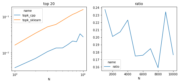
import matplotlib.pyplot as plt

fig, ax = plt.subplots(1, 2, figsize=(10, 4))
piv = df.pivot("N", "name", "average")
piv.plot(ax=ax[0], logy=True, logx=True)
ax[0].set_title("top 20")
piv["ratio"] = piv["topk_cpp"] / piv["topk_sklearn"]
piv[["ratio"]].plot(ax=ax[1])
ax[1].set_title("ratio");

Speed comparison by k

rows = []
X = rnd.randn(2000, 1000)
for k in tqdm(list(range(1, 20)) + list(range(20, 1000, 20))):
    res = measure_time('topk_sklearn(X, k)',
                       {'X': X, 'topk_sklearn': topk_sklearn, 'k': k},
                       div_by_number=True,
                       number=2, repeat=2)
    res["k"] = k
    res["name"] = 'topk_sklearn'
    rows.append(res)
    res = measure_time('topk_cpp(X, k)',
                       {'X': X, 'topk_cpp': topk_cpp, 'k': k},
                       div_by_number=True,
                       number=2, repeat=2)
    res["k"] = k
    res["name"] = 'topk_cpp'
    rows.append(res)

df = DataFrame(rows)
df.head()

100%|██████████| 68/68 [00:34<00:00,  1.95it/s]

	average	deviation	min_exec	max_exec	repeat	number	context_size	k	name
0	0.009558	0.001392	0.008166	0.010949	2	2	240	1	topk_sklearn
1	0.002665	0.000571	0.002094	0.003236	2	2	240	1	topk_cpp
2	0.021933	0.000575	0.021358	0.022508	2	2	240	2	topk_sklearn
3	0.001000	0.000084	0.000917	0.001084	2	2	240	2	topk_cpp
4	0.025986	0.001411	0.024575	0.027398	2	2	240	3	topk_sklearn

fig, ax = plt.subplots(1, 2, figsize=(10, 4))
piv = df.pivot("k", "name", "average")
piv.plot(ax=ax[0], logy=True, logx=True)
ax[0].set_title("top k for 2000 rows")
piv["ratio"] = piv["topk_cpp"] / piv["topk_sklearn"]
piv[["ratio"]].plot(ax=ax[1])
ax[1].set_title("ratio")
ax[0].set_xlabel("k")
ax[1].set_xlabel("k");

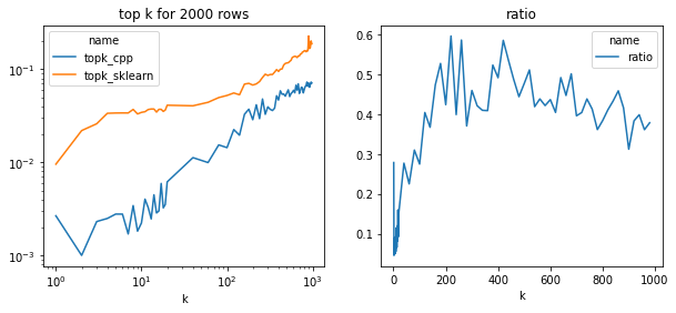
The implementation is half faster in all cases and much more efficient for small values which is usually the case for the nearest neighbors. This implementation is using openmp, maybe that’s why it gets 50% faster on this two cores machine.