NeuralTreeNet et coût

Links: notebook, html, PDF, python, slides, GitHub

La classe NeuralTreeNet convertit un arbre de décision en réseau de neurones. Si la conversion n’est pas exacte mais elle permet d’obtenir un modèle différentiable et apprenable avec un algorithme d’optimisation à base de gradient. Ce notebook compare le temps d’éxécution entre un arbre et le réseau de neurones.

from jyquickhelper import add_notebook_menu
add_notebook_menu()

%matplotlib inline

%load_ext mlprodict

Jeux de données

On construit un jeu de données aléatoire.

import numpy

X = numpy.random.randn(10000, 10)
y = X.sum(axis=1) / X.shape[1]
X = X.astype(numpy.float64)
y = y.astype(numpy.float64)

middle = X.shape[0] // 2
X_train, X_test = X[:middle], X[middle:]
y_train, y_test = y[:middle], y[middle:]

Caler un arbre de décision

from sklearn.tree import DecisionTreeRegressor

tree = DecisionTreeRegressor(max_depth=7)
tree.fit(X_train, y_train)
tree.score(X_train, y_train), tree.score(X_test, y_test)

(0.6091161526814477, 0.3884519134946681)

from sklearn.metrics import r2_score
r2_score(y_test, tree.predict(X_test))

0.3884519134946681

Covnersion de l’arbre en réseau de neurones

from pandas import DataFrame
from mlstatpy.ml.neural_tree import NeuralTreeNet, NeuralTreeNetRegressor

xe = X_test.astype(numpy.float32)
expected = tree.predict(xe)

nn = NeuralTreeNetRegressor(NeuralTreeNet.create_from_tree(tree, arch='compact'))
got = nn.predict(xe)
me = numpy.abs(got - expected).mean()
mx = numpy.abs(got - expected).max()
DataFrame([{"average absolute error": me, "max absolute error": mx}]).T

	0
average absolute error	0.210314
max absolute error	1.679553

La conversion est loin d’être parfaite. La raison vient du fait que les fonctions de seuil sont approchées par des fonctions sigmoïdes. Il suffit d’une erreur minime pour que la décision prenne un chemin différent dans l’arbre et soit complètement différente.

Conversion au format ONNX

from mlprodict.onnx_conv import to_onnx

onx_tree = to_onnx(tree, X[:1].astype(numpy.float32))
onx_nn = to_onnx(nn, X[:1].astype(numpy.float32))

Le réseau de neurones peut être représenté comme suit.

%onnxview onx_nn

from mlprodict.plotting.text_plot import onnx_simple_text_plot
print(onnx_simple_text_plot(onx_nn))

opset: domain='' version=15
input: name='X' type=dtype('float32') shape=[None, 10]
init: name='Ma_MatMulcst' type=dtype('float32') shape=(1270,)
init: name='Ad_Addcst' type=dtype('float32') shape=(127,)
init: name='Mu_Mulcst' type=dtype('float32') shape=(1,) -- array([4.], dtype=float32)
init: name='Ma_MatMulcst1' type=dtype('float32') shape=(16256,)
init: name='Ad_Addcst1' type=dtype('float32') shape=(128,)
init: name='Ma_MatMulcst2' type=dtype('float32') shape=(128,)
init: name='Ad_Addcst2' type=dtype('float32') shape=(1,) -- array([0.], dtype=float32)
MatMul(X, Ma_MatMulcst) -> Ma_Y02
  Add(Ma_Y02, Ad_Addcst) -> Ad_C02
    Mul(Ad_C02, Mu_Mulcst) -> Mu_C01
      Sigmoid(Mu_C01) -> Si_Y01
        MatMul(Si_Y01, Ma_MatMulcst1) -> Ma_Y01
          Add(Ma_Y01, Ad_Addcst1) -> Ad_C01
            Mul(Ad_C01, Mu_Mulcst) -> Mu_C0
              Sigmoid(Mu_C0) -> Si_Y0
                MatMul(Si_Y0, Ma_MatMulcst2) -> Ma_Y0
                  Add(Ma_Y0, Ad_Addcst2) -> Ad_C0
                    Identity(Ad_C0) -> variable
output: name='variable' type=dtype('float32') shape=[None, 1]

Temps de calcul des prédictions

from mlprodict.onnxrt import OnnxInference

oinf_tree = OnnxInference(onx_tree, runtime='onnxruntime1')
oinf_nn = OnnxInference(onx_nn, runtime='onnxruntime1')

%timeit tree.predict(xe)

No CUDA runtime is found, using CUDA_HOME='C:Program FilesNVIDIA GPU Computing ToolkitCUDAv11.5'
518 µs ± 41.4 µs per loop (mean ± std. dev. of 7 runs, 1,000 loops each)

%timeit oinf_tree.run({'X': xe})

124 µs ± 5.21 µs per loop (mean ± std. dev. of 7 runs, 10,000 loops each)

%timeit oinf_nn.run({'X': xe})

3.18 ms ± 569 µs per loop (mean ± std. dev. of 7 runs, 100 loops each)

Le temps de calcul est nettement plus long pour le réseau de neurones. Si l’arbre de décision a une profondeur de d, l’arbre de décision va faire exactement d comparaisons. Le réseau de neurones quant à lui évalue tous les seuils pour chaque prédiction, soit . Vérifions cela en faisant variable la profondeur.

Temps de calcul en fonction de la profondeur

from tqdm import tqdm
from cpyquickhelper.numbers import measure_time

data = []
for d in tqdm(range(2, 10)):
    tree = DecisionTreeRegressor(max_depth=d)
    tree.fit(X_train, y_train)
    obs = measure_time(lambda: tree.predict(xe), number=20, repeat=20)
    obs.update(dict(d=d, exp='skl'))
    data.append(obs)

    nn = NeuralTreeNetRegressor(NeuralTreeNet.create_from_tree(tree, arch='compact'))

    onx_tree = to_onnx(tree, X[:1].astype(numpy.float32))
    onx_nn = to_onnx(nn, X[:1].astype(numpy.float32))
    oinf_tree = OnnxInference(onx_tree, runtime='onnxruntime1')
    oinf_nn = OnnxInference(onx_nn, runtime='onnxruntime1')

    obs = measure_time(lambda: oinf_tree.run({'X': xe}), number=10, repeat=10)
    obs.update(dict(d=d, exp='onx_tree'))
    data.append(obs)

    obs = measure_time(lambda: oinf_nn.run({'X': xe}), number=10, repeat=10)
    obs.update(dict(d=d, exp='onx_nn'))
    data.append(obs)

df = DataFrame(data)
df

100%|██████████| 8/8 [00:07<00:00,  1.04it/s]

	average	deviation	min_exec	max_exec	repeat	number	ttime	context_size	d	exp
0	0.005656	0.001292	0.004990	0.009533	20	20	0.113116	64	2	skl
1	0.000609	0.000084	0.000538	0.000830	10	10	0.006088	64	2	onx_tree
2	0.002337	0.000563	0.001737	0.003299	10	10	0.023374	64	2	onx_nn
3	0.005607	0.000962	0.004669	0.007374	20	20	0.112131	64	3	skl
4	0.000709	0.000240	0.000534	0.001363	10	10	0.007087	64	3	onx_tree
5	0.002506	0.000448	0.002073	0.003736	10	10	0.025064	64	3	onx_nn
6	0.006398	0.000942	0.005576	0.009556	20	20	0.127961	64	4	skl
7	0.000852	0.000335	0.000633	0.001715	10	10	0.008519	64	4	onx_tree
8	0.004151	0.000763	0.003408	0.005826	10	10	0.041507	64	4	onx_nn
9	0.007266	0.000731	0.006400	0.009247	20	20	0.145314	64	5	skl
10	0.000963	0.000169	0.000826	0.001327	10	10	0.009634	64	5	onx_tree
11	0.006113	0.000560	0.005360	0.007255	10	10	0.061134	64	5	onx_nn
12	0.008881	0.001234	0.007601	0.012340	20	20	0.177622	64	6	skl
13	0.001175	0.000613	0.000815	0.002984	10	10	0.011754	64	6	onx_tree
14	0.011537	0.001079	0.010146	0.013582	10	10	0.115367	64	6	onx_nn
15	0.011134	0.000887	0.009569	0.013273	20	20	0.222676	64	7	skl
16	0.001399	0.000131	0.001301	0.001742	10	10	0.013988	64	7	onx_tree
17	0.034831	0.004986	0.027853	0.046760	10	10	0.348306	64	7	onx_nn
18	0.011263	0.001060	0.009911	0.013893	20	20	0.225251	64	8	skl
19	0.001226	0.000148	0.001033	0.001609	10	10	0.012259	64	8	onx_tree
20	0.141722	0.051041	0.089979	0.270129	10	10	1.417218	64	8	onx_nn
21	0.016436	0.004827	0.011379	0.028261	20	20	0.328716	64	9	skl
22	0.003879	0.001963	0.002402	0.008579	10	10	0.038786	64	9	onx_tree
23	0.323764	0.063045	0.261038	0.456420	10	10	3.237635	64	9	onx_nn

piv = df.pivot('d', 'exp', 'average')
piv.plot(logy=True, title="Temps de calcul en fonction de la profondeur");

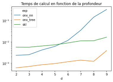
L’hypothèse est vérifiée.