Analyse de survie
Links: notebook html , PDF python slides , GitHub
from jyquickhelper import add_notebook_menu
add_notebook_menu ()
On récupère les données disponibles sur open.data.gouv.fr Données
hospitalières relatives à l’épidémie de
COVID-19 .
Ces données ne permettent pas de construire la courbe de
Kaplan-Meier .
On sait combien de personnes rentrent et sortent chaque jour mais on ne
sait pas quand une personne qui sort un 1er avril est entrée.
import numpy.random as rnd
import pandas
df = pandas . read_csv ( "https://www.data.gouv.fr/en/datasets/r/63352e38-d353-4b54-bfd1-f1b3ee1cabd7" , sep = ";" )
gr = df [[ "jour" , "rad" , "dc" ]] . groupby ([ "jour" ]) . sum ()
diff = gr . diff () . reset_index ( drop = False )
diff . head ()
jour
rad
dc
0
2020-03-18
NaN
NaN
1
2020-03-19
695.0
207.0
2
2020-03-20
806.0
248.0
3
2020-03-21
452.0
151.0
4
2020-03-22
608.0
210.0
def donnees_artificielles ( hosp , mu = 14 , nu = 21 ):
dt = pandas . to_datetime ( hosp [ 'jour' ])
res = []
for i in range ( hosp . shape [ 0 ]):
date = dt [ i ] . dayofyear
h = hosp . iloc [ i , 1 ]
delay = rnd . exponential ( mu , int ( h ))
for j in range ( delay . shape [ 0 ]):
res . append ([ date - int ( delay [ j ]), date , 1 ])
h = hosp . iloc [ i , 2 ]
delay = rnd . exponential ( nu , int ( h ))
for j in range ( delay . shape [ 0 ]):
res . append ([ date - int ( delay [ j ]), date , 0 ])
return pandas . DataFrame ( res , columns = [ "entree" , "sortie" , "issue" ])
data = donnees_artificielles ( diff [ 1 :] . reset_index ( drop = True )) . sort_values ( 'entree' )
data . head ()
entree
sortie
issue
518488
-200
19
0
541408
-192
27
0
476735
-187
2
0
587013
-185
42
0
476057
-180
1
0
Chaque ligne est une personne, entree sortie issue
entree
sortie
issue
count
624130.000000
624130.000000
624130.000000
mean
169.704510
184.532815
0.806729
std
125.420957
124.343186
0.394864
min
-200.000000
1.000000
0.000000
25%
53.000000
84.000000
1.000000
50%
133.000000
144.000000
1.000000
75%
301.000000
315.000000
1.000000
max
366.000000
366.000000
1.000000
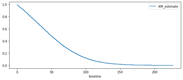
Il y a environ 80% de survie dans ces données.
import numpy
duree = data . sortie - data . entree
deces = ( data . issue == 0 ) . astype ( numpy . int32 )
import numpy
import matplotlib.pyplot as plt
from lifelines import KaplanMeierFitter
fig , ax = plt . subplots ( 1 , 1 , figsize = ( 10 , 4 ))
kmf = KaplanMeierFitter ()
kmf . fit ( duree , deces )
kmf . plot ( ax = ax )
ax . legend ();
On reprend les données artificiellement générées et on ajoute une
variable identique à la durée plus un bruit mais quasi nul
import pandas
data_simple = pandas . DataFrame ({ 'duree' : duree , 'deces' : deces ,
'X1' : duree * 0.57 * deces + numpy . random . randn ( duree . shape [ 0 ]),
'X2' : duree * ( - 0.57 ) * deces + numpy . random . randn ( duree . shape [ 0 ])})
data_simple . head ()
duree
deces
X1
X2
518488
219
1
125.653230
-125.666662
541408
219
1
126.006024
-125.327549
476735
189
1
107.920779
-108.358230
587013
227
1
129.788930
-130.045019
476057
181
1
103.642440
-103.793008
from sklearn.model_selection import train_test_split
data_train , data_test = train_test_split ( data_simple , test_size = 0.8 )
from lifelines.fitters.coxph_fitter import CoxPHFitter
cox = CoxPHFitter ()
cox . fit ( data_train [[ 'duree' , 'deces' , 'X1' ]], duration_col = "duree" , event_col = "deces" ,
show_progress = True )
Iteration 1 : norm_delta = 0.13943 , step_size = 0.9000 , log_lik = - 250658.36250 , newton_decrement = 889.93933 , seconds_since_start = 0.0
Iteration 2 : norm_delta = 0.00660 , step_size = 0.9000 , log_lik = - 249862.37270 , newton_decrement = 2.81312 , seconds_since_start = 0.0
Iteration 3 : norm_delta = 0.00073 , step_size = 0.9000 , log_lik = - 249859.57376 , newton_decrement = 0.03357 , seconds_since_start = 0.1
Iteration 4 : norm_delta = 0.00000 , step_size = 1.0000 , log_lik = - 249859.54017 , newton_decrement = 0.00000 , seconds_since_start = 0.1
Convergence success after 4 iterations .
< lifelines . CoxPHFitter : fitted with 124826 total observations , 100754 right - censored observations >
model
lifelines.CoxPHFitter
duration col
'duree'
event col
'deces'
baseline estimation
breslow
number of observations
124826
number of events observed
24072
partial log-likelihood
-249859.54
time fit was run
2021-02-24 23:48:57 UTC
coef
exp(coef)
se(coef)
coef lower 95%
coef upper 95%
exp(coef) lower 95%
exp(coef) upper 95%
z
p
-log2(p)
X1
0.02
1.02
0.00
0.02
0.02
1.02
1.02
42.23
<0.005
inf
Concordance
0.69
Partial AIC
499721.08
log-likelihood ratio test
1597.64 on 1 df
-log2(p) of ll-ratio test
inf
cox2 = CoxPHFitter ()
cox2 . fit ( data_train [[ 'duree' , 'deces' , 'X2' ]], duration_col = "duree" , event_col = "deces" ,
show_progress = True )
cox2 . print_summary ()
Iteration 1 : norm_delta = 0.13946 , step_size = 0.9000 , log_lik = - 250658.36250 , newton_decrement = 888.92089 , seconds_since_start = 0.0
Iteration 2 : norm_delta = 0.00667 , step_size = 0.9000 , log_lik = - 249863.61089 , newton_decrement = 2.86434 , seconds_since_start = 0.0
Iteration 3 : norm_delta = 0.00074 , step_size = 0.9000 , log_lik = - 249860.76079 , newton_decrement = 0.03426 , seconds_since_start = 0.1
Iteration 4 : norm_delta = 0.00000 , step_size = 1.0000 , log_lik = - 249860.72650 , newton_decrement = 0.00000 , seconds_since_start = 0.1
Convergence success after 4 iterations .
model
lifelines.CoxPHFitter
duration col
'duree'
event col
'deces'
baseline estimation
breslow
number of observations
124826
number of events observed
24072
partial log-likelihood
-249860.73
time fit was run
2021-02-24 23:48:59 UTC
coef
exp(coef)
se(coef)
coef lower 95%
coef upper 95%
exp(coef) lower 95%
exp(coef) upper 95%
z
p
-log2(p)
X2
-0.02
0.98
0.00
-0.02
-0.02
0.98
0.98
-42.21
<0.005
inf
Concordance
0.69
Partial AIC
499723.45
log-likelihood ratio test
1595.27 on 1 df
-log2(p) of ll-ratio test
inf
cox . predict_cumulative_hazard ( data_test [: 5 ])
621725
110352
139986
72623
248121
0.0
0.008806
0.008673
0.008543
0.008717
0.008661
1.0
0.018218
0.017942
0.017673
0.018035
0.017918
2.0
0.026735
0.026330
0.025936
0.026466
0.026295
3.0
0.036002
0.035457
0.034926
0.035640
0.035409
4.0
0.045543
0.044854
0.044182
0.045085
0.044793
...
...
...
...
...
...
184.0
2.055736
2.024623
1.994277
2.035070
2.021872
189.0
2.092002
2.060340
2.029459
2.070971
2.057541
197.0
2.138687
2.106318
2.074747
2.117186
2.103457
201.0
2.205513
2.172133
2.139576
2.183341
2.169182
217.0
2.330629
2.295356
2.260952
2.307199
2.292237
165 rows × 5 columns
cox . predict_survival_function ( data_test [: 5 ])
621725
110352
139986
72623
248121
0.0
0.991233
0.991365
0.991494
0.991321
0.991377
1.0
0.981947
0.982218
0.982482
0.982127
0.982242
2.0
0.973619
0.974013
0.974398
0.973881
0.974048
3.0
0.964638
0.965164
0.965677
0.964988
0.965211
4.0
0.955478
0.956137
0.956780
0.955916
0.956196
...
...
...
...
...
...
184.0
0.127999
0.132044
0.136112
0.130671
0.132407
189.0
0.123440
0.127411
0.131407
0.126063
0.127768
197.0
0.117809
0.121685
0.125588
0.120370
0.122034
201.0
0.110194
0.113934
0.117705
0.112664
0.114271
217.0
0.097235
0.100726
0.104251
0.099540
0.101040
165 rows × 5 columns