Batch predictions without parallelization

The goal is to compare the processing time for batch predictions with onnxruntime and lightgbm without any parallelization. It compares the implementations.

Train a LGBMRegressor

import warnings
import time
import os
from packaging.version import Version
import numpy
from pandas import DataFrame
import onnx
import matplotlib.pyplot as plt
from tqdm import tqdm
from lightgbm import LGBMRegressor, Booster
from onnxruntime import InferenceSession, SessionOptions, ExecutionMode
from skl2onnx import update_registered_converter, to_onnx
from skl2onnx.common.shape_calculator import calculate_linear_regressor_output_shapes  # noqa
from onnxmltools import __version__ as oml_version
from onnxmltools.convert.lightgbm.operator_converters.LightGbm import convert_lightgbm  # noqa
from mlprodict.onnxrt import OnnxInference


def skl2onnx_convert_lightgbm(scope, operator, container):
    options = scope.get_options(operator.raw_operator)
    if 'split' in options:
        if Version(oml_version) < Version('1.9.2'):
            warnings.warn(
                "Option split was released in version 1.9.2 but %s is "
                "installed. It will be ignored." % oml_version)
        operator.split = options['split']
    else:
        operator.split = None
    convert_lightgbm(scope, operator, container)


update_registered_converter(
    LGBMRegressor, 'LightGbmLGBMRegressor',
    calculate_linear_regressor_output_shapes,
    skl2onnx_convert_lightgbm,
    options={'split': None})

N = 1000
Ntrees = [10, 100, 200]
X = numpy.random.randn(N, 1000)
y = (numpy.random.randn(N) +
     numpy.random.randn(N) * 100 * numpy.random.randint(0, 1, N))

filenames = [f"plot_lightgbm_regressor_{nt}_{X.shape[1]}.onnx"
             for nt in Ntrees]

regs = []
models_onnx = []
for nt, filename in zip(Ntrees, filenames):
    if not os.path.exists(filename) or not os.path.exists(filename + ".txt"):
        print(f"training with shape={X.shape} and {nt} trees")
        r = LGBMRegressor(n_estimators=nt, max_depth=10).fit(X, y)
        r.booster_.save_model(filename + ".txt")
        print("done.")

        model_onnx = to_onnx(r, X[:1].astype(numpy.float32),
                             target_opset={'': 17, 'ai.onnx.ml': 1})
        models_onnx.append(model_onnx)
        with open(filename, "wb") as f:
            f.write(model_onnx.SerializeToString())
    else:
        with open(filename, "rb") as f:
            model_onnx = onnx.load(f)
        models_onnx.append(model_onnx)
    r = Booster(model_file=filename + ".txt", params=dict(num_threads=1))
    regs.append(r)

training with shape=(1000, 1000) and 10 trees
done.
training with shape=(1000, 1000) and 100 trees
done.
training with shape=(1000, 1000) and 200 trees
done.

Convert

We convert the same model following the two scenarios, one single TreeEnsembleRegressor node, or more. split parameter is the number of trees per node TreeEnsembleRegressor.

opts = SessionOptions()
opts.execution_mode = ExecutionMode.ORT_SEQUENTIAL
opts.inter_op_num_threads = 1
opts.intra_op_num_threads = 1
sesss = [InferenceSession(m.SerializeToString(),
                          providers=['CPUExecutionProvider'],
                          sess_options=opts)
         for m in models_onnx]

# a different engine, disable the parallelism
oinfs = [OnnxInference(m) for m in models_onnx]
for oinf in oinfs:
    oinf.sequence_[0].ops_.change_parallel(100000, 100000, 100000)

Processing time

repeat = 9
data = []
for N in tqdm([1, 2, 5] + list(range(10, 100, 10)) +
              list(range(100, 1201, 100))):

    X32 = numpy.random.randn(N, X.shape[1]).astype(numpy.float32)
    obs = dict(N=N)
    for sess, oinf, r, T in zip(sesss, oinfs, regs, Ntrees):
        # lightgbm
        times = []
        for _ in range(repeat):
            begin = time.perf_counter()
            r.predict(X32, num_threads=1)
            end = time.perf_counter() - begin
            times.append(end / X32.shape[0])
        times.sort()
        obs[f"batch-lgbm-{T}"] = sum(times[2:-2]) / (len(times) - 4)

        # onnxruntime
        times = []
        for _ in range(repeat):
            begin = time.perf_counter()
            sess.run(None, {'X': X32})
            end = time.perf_counter() - begin
            times.append(end / X32.shape[0])
        times.sort()
        obs[f"batch-ort-{T}"] = sum(times[2:-2]) / (len(times) - 4)

        # OnnxInference
        times = []
        for _ in range(repeat):
            begin = time.perf_counter()
            oinf.run({'X': X32})
            end = time.perf_counter() - begin
            times.append(end / X32.shape[0])
        times.sort()
        obs[f"batch-oinf-{T}"] = sum(times[2:-2]) / (len(times) - 4)

        data.append(obs)

df = DataFrame(data).set_index("N")
df.reset_index(drop=False).to_csv(
    "plot_gexternal_lightgbm_reg_mono.csv", index=False)
print(df)

  0%|          | 0/24 [00:00<?, ?it/s]
 21%|##        | 5/24 [00:00<00:00, 33.88it/s]
 38%|###7      | 9/24 [00:00<00:00, 15.10it/s]
 46%|####5     | 11/24 [00:00<00:01, 11.63it/s]
 54%|#####4    | 13/24 [00:01<00:01,  9.09it/s]
 62%|######2   | 15/24 [00:02<00:01,  4.81it/s]
 67%|######6   | 16/24 [00:02<00:02,  3.19it/s]
 71%|#######   | 17/24 [00:03<00:03,  2.16it/s]
 75%|#######5  | 18/24 [00:05<00:03,  1.53it/s]
 79%|#######9  | 19/24 [00:06<00:04,  1.14it/s]
 83%|########3 | 20/24 [00:08<00:04,  1.12s/it]
 88%|########7 | 21/24 [00:10<00:04,  1.37s/it]
 92%|#########1| 22/24 [00:13<00:03,  1.63s/it]
 96%|#########5| 23/24 [00:15<00:01,  1.90s/it]
100%|##########| 24/24 [00:18<00:00,  2.15s/it]
100%|##########| 24/24 [00:18<00:00,  1.30it/s]
      batch-lgbm-10  batch-ort-10  ...  batch-ort-200  batch-oinf-200
N                                  ...
1          0.000262      0.000042  ...       0.000081        0.000106
1          0.000262      0.000042  ...       0.000081        0.000106
1          0.000262      0.000042  ...       0.000081        0.000106
2          0.000140      0.000022  ...       0.000076        0.000082
2          0.000140      0.000022  ...       0.000076        0.000082
...             ...           ...  ...            ...             ...
1100       0.000013      0.000004  ...       0.000075        0.000036
1100       0.000013      0.000004  ...       0.000075        0.000036
1200       0.000013      0.000004  ...       0.000074        0.000036
1200       0.000013      0.000004  ...       0.000074        0.000036
1200       0.000013      0.000004  ...       0.000074        0.000036

[72 rows x 9 columns]

Plots.

fig, ax = plt.subplots(1, 3, figsize=(12, 4))

for i, T in enumerate(Ntrees):
    df[[f"batch-ort-{T}", f"batch-oinf-{T}",
        f"batch-lgbm-{T}"]].plot(
        ax=ax[i], logy=True, logx=True,
        title=f"Processing time per observation (1 thread)\n{T} Trees")

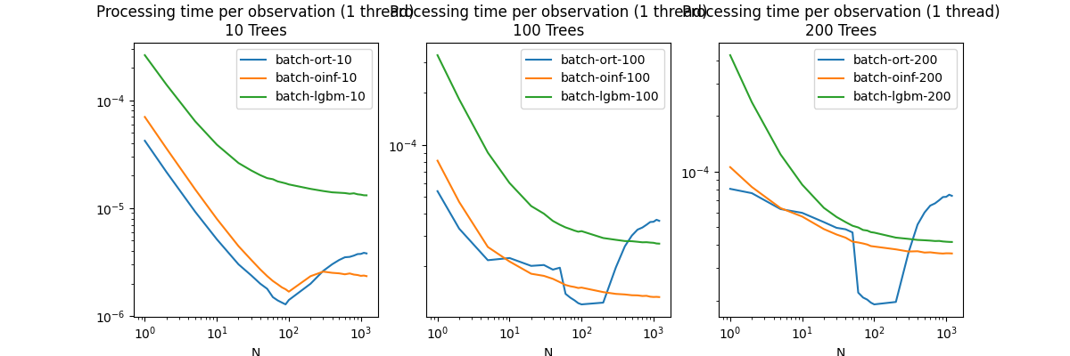
Conclusion

The first graph shows a huge drop the prediction time by batch. It means the parallelization is triggered. It may have been triggered sooner on this machine but this decision could be different on another one. An approach like the one TVM chose could be a good answer. If the model must be fast, then it is worth benchmarking many strategies to parallelize until the best one is found on a specific machine.

# plt.show()