Batch predictions vs one-off predictions

The goal is to compare the processing time between batch predictions and one-off prediction for the same number of predictions on trees. onnxruntime parallelizes the prediction by trees or by rows. The rule is fixed and cannot be changed but it seems to have some loopholes.

Train a LGBMRegressor

import warnings
import time
import os
from packaging.version import Version
import numpy
from pandas import DataFrame
import onnx
import matplotlib.pyplot as plt
from tqdm import tqdm
from lightgbm import LGBMRegressor
from onnxruntime import InferenceSession
from skl2onnx import update_registered_converter, to_onnx
from skl2onnx.common.shape_calculator import calculate_linear_regressor_output_shapes  # noqa
from onnxmltools import __version__ as oml_version
from onnxmltools.convert.lightgbm.operator_converters.LightGbm import convert_lightgbm  # noqa


N = 1000
Ntrees = [10, 100, 200]
X = numpy.random.randn(N, 1000)
y = (numpy.random.randn(N) +
     numpy.random.randn(N) * 100 * numpy.random.randint(0, 1, N))

filenames = [f"plot_lightgbm_regressor_{nt}_{X.shape[1]}.onnx"
             for nt in Ntrees]

regs = []
for nt, filename in zip(Ntrees, filenames):
    if not os.path.exists(filename):
        print(f"training with shape={X.shape} and {nt} trees")
        r = LGBMRegressor(n_estimators=nt).fit(X, y)
        regs.append(r)
        print("done.")
    else:
        regs.append(None)

training with shape=(1000, 1000) and 10 trees
done.
training with shape=(1000, 1000) and 100 trees
done.
training with shape=(1000, 1000) and 200 trees
done.

Register the converter for LGBMRegressor

def skl2onnx_convert_lightgbm(scope, operator, container):
    options = scope.get_options(operator.raw_operator)
    if 'split' in options:
        if Version(oml_version) < Version('1.9.2'):
            warnings.warn(
                "Option split was released in version 1.9.2 but %s is "
                "installed. It will be ignored." % oml_version)
        operator.split = options['split']
    else:
        operator.split = None
    convert_lightgbm(scope, operator, container)


update_registered_converter(
    LGBMRegressor, 'LightGbmLGBMRegressor',
    calculate_linear_regressor_output_shapes,
    skl2onnx_convert_lightgbm,
    options={'split': None})

Convert

We convert the same model following the two scenarios, one single TreeEnsembleRegressor node, or more. split parameter is the number of trees per node TreeEnsembleRegressor.

models_onnx = []
for i, filename in enumerate(filenames):
    print(i, filename)
    if os.path.exists(filename):
        with open(filename, "rb") as f:
            model_onnx = onnx.load(f)
        models_onnx.append(model_onnx)
    else:
        model_onnx = to_onnx(regs[i], X[:1].astype(numpy.float32),
                             target_opset={'': 17, 'ai.onnx.ml': 3})
        models_onnx.append(model_onnx)
        with open(filename, "wb") as f:
            f.write(model_onnx.SerializeToString())

sesss = [InferenceSession(m.SerializeToString(),
                          providers=['CPUExecutionProvider'])
         for m in models_onnx]

0 plot_lightgbm_regressor_10_1000.onnx
1 plot_lightgbm_regressor_100_1000.onnx
2 plot_lightgbm_regressor_200_1000.onnx

Processing time

repeat = 7
data = []
for N in tqdm(list(range(10, 100, 10)) +
              list(range(100, 1000, 100)) +
              list(range(1000, 10001, 1000))):

    X32 = numpy.random.randn(N, X.shape[1]).astype(numpy.float32)
    obs = dict(N=N)
    for sess, T in zip(sesss, Ntrees):
        times = []
        for _ in range(repeat):
            begin = time.perf_counter()
            sess.run(None, {'X': X32})
            end = time.perf_counter() - begin
            times.append(end / X32.shape[0])
        times.sort()
        obs[f"batch-{T}"] = sum(times[2:-2]) / (len(times) - 4)

        times = []
        for _ in range(repeat):
            begin = time.perf_counter()
            for i in range(X32.shape[0]):
                sess.run(None, {'X': X32[i: i + 1]})
            end = time.perf_counter() - begin
            times.append(end / X32.shape[0])
        times.sort()
        obs[f"one-off-{T}"] = sum(times[2:-2]) / (len(times) - 4)
    data.append(obs)

df = DataFrame(data).set_index("N")
df.reset_index(drop=False).to_csv(
    "plot_gexternal_lightgbm_reg_per.csv", index=False)
print(df)

  0%|          | 0/28 [00:00<?, ?it/s]
 11%|#         | 3/28 [00:00<00:01, 19.72it/s]
 18%|#7        | 5/28 [00:00<00:01, 13.27it/s]
 25%|##5       | 7/28 [00:00<00:02,  9.79it/s]
 32%|###2      | 9/28 [00:00<00:02,  8.30it/s]
 36%|###5      | 10/28 [00:01<00:02,  7.56it/s]
 39%|###9      | 11/28 [00:01<00:02,  5.89it/s]
 43%|####2     | 12/28 [00:01<00:03,  4.27it/s]
 46%|####6     | 13/28 [00:02<00:04,  3.00it/s]
 50%|#####     | 14/28 [00:03<00:06,  2.25it/s]
 54%|#####3    | 15/28 [00:04<00:07,  1.74it/s]
 57%|#####7    | 16/28 [00:05<00:08,  1.41it/s]
 61%|######    | 17/28 [00:06<00:09,  1.18it/s]
 64%|######4   | 18/28 [00:07<00:09,  1.01it/s]
 68%|######7   | 19/28 [00:09<00:10,  1.13s/it]
 71%|#######1  | 20/28 [00:12<00:13,  1.65s/it]
 75%|#######5  | 21/28 [00:16<00:17,  2.45s/it]
 79%|#######8  | 22/28 [00:22<00:20,  3.44s/it]
 82%|########2 | 23/28 [00:29<00:22,  4.56s/it]
 86%|########5 | 24/28 [00:37<00:23,  5.78s/it]
 89%|########9 | 25/28 [00:48<00:21,  7.08s/it]
 93%|#########2| 26/28 [00:59<00:16,  8.41s/it]
 96%|#########6| 27/28 [01:12<00:09,  9.77s/it]
100%|##########| 28/28 [01:26<00:00, 11.14s/it]
100%|##########| 28/28 [01:26<00:00,  3.10s/it]
           batch-10  one-off-10  batch-100  one-off-100  batch-200  one-off-200
N
10     5.256629e-06    0.000045   0.000025     0.000057   0.000075     0.000167
20     3.236299e-06    0.000045   0.000023     0.000058   0.000066     0.000063
30     2.438310e-06    0.000046   0.000022     0.000074   0.000064     0.000070
40     2.094317e-06    0.000046   0.000022     0.000066   0.000062     0.000086
50     1.906313e-06    0.000046   0.000021     0.000063   0.000060     0.000097
60     1.416150e-06    0.000046   0.000004     0.000075   0.000026     0.000075
70     1.145758e-06    0.000046   0.000014     0.000071   0.000007     0.000070
80     1.043154e-06    0.000046   0.000003     0.000065   0.000025     0.000090
90     9.499516e-07    0.000046   0.000005     0.000074   0.000009     0.000106
100    9.174897e-07    0.000046   0.000003     0.000066   0.000023     0.000103
200    7.846750e-07    0.000046   0.000003     0.000058   0.000004     0.000084
300    1.008190e-06    0.000047   0.000004     0.000058   0.000006     0.000066
400    1.126488e-06    0.000047   0.000005     0.000058   0.000037     0.000063
500    1.132216e-06    0.000047   0.000005     0.000059   0.000023     0.000063
600    1.152744e-06    0.000047   0.000006     0.000059   0.000024     0.000064
700    1.160712e-06    0.000047   0.000006     0.000058   0.000024     0.000064
800    1.184026e-06    0.000047   0.000006     0.000058   0.000022     0.000064
900    1.151270e-06    0.000047   0.000006     0.000058   0.000018     0.000063
1000   1.128798e-06    0.000047   0.000006     0.000059   0.000016     0.000064
2000   1.025395e-06    0.000047   0.000006     0.000059   0.000014     0.000064
3000   9.748289e-07    0.000047   0.000006     0.000058   0.000015     0.000064
4000   9.530169e-07    0.000047   0.000006     0.000059   0.000015     0.000064
5000   9.424797e-07    0.000047   0.000006     0.000059   0.000015     0.000064
6000   9.153984e-07    0.000047   0.000006     0.000059   0.000015     0.000064
7000   9.050845e-07    0.000047   0.000006     0.000059   0.000016     0.000064
8000   9.103698e-07    0.000047   0.000006     0.000058   0.000016     0.000064
9000   9.047970e-07    0.000047   0.000006     0.000058   0.000016     0.000064
10000  8.911956e-07    0.000047   0.000006     0.000058   0.000016     0.000063

Plots.

fig, ax = plt.subplots(1, 3, figsize=(12, 4))

for i, T in enumerate(Ntrees):
    df[[f"batch-{T}", f"one-off-{T}"]].plot(
        ax=ax[i], title=f"Processing time per observation\n{T} Trees",
        logy=True, logx=True)

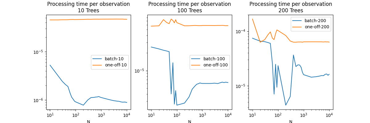
Conclusion

The first graph shows a huge drop the prediction time by batch. It means the parallelization is triggered. It may have been triggered sooner on this machine but this decision could be different on another one. An approach like the one TVM chose could be a good answer. If the model must be fast, then it is worth benchmarking many strategies to parallelize until the best one is found on a specific machine.

# plt.show()