Partial Training with OrtGradientForwardBackwardOptimizer#
Design#
Section Full Training with OrtGradientOptimizer introduces a class able to train an ONNX graph. onnxruntime-training handles the computation of the loss, the gradient. It updates the weights as well. This design does not work when ONNX graph only plays a part in the model and is not the whole model. A deep neural network could be composed with a first layer from torch, a second layer from ONNX, and be trained by a gradient descent implemented in python.
Partial training is another way to train an ONNX model. It can be trained
as a standalone ONNX graph or be integrated in a torch model or any
framework implementing forward and backward mechanism.
It leverages class TrainingAgent from onnxruntime-training.
However a couple of lines of code are not enough to use this class.
This package defines a class implementing the missing pieces:
OrtGradientForwardBackwardOptimizer.
It is initialized with an ONNX graph defining a prediction function.
train_session = OrtGradientForwardBackwardOptimizer(
    onx, ['coef', 'intercept'],
    learning_rate=LearningRateSGDNesterov(),
    learning_loss=ElasticLearningLoss(l1_weight=0.1, l2_weight=0.9),
    learning_penalty=ElasticLearningPenalty(l1=0.1, l2=0.9))
The class uses onnxruntime-training to build two others, one to predict with custom weights (and not initializers), another to compute the gradient. It implements forward and backward as explained in section l-orttraining-second-api.
In addition the class holds three attributes defining the loss, its gradient, the regularization, its gradient, a learning rate possibly with momentum. They are not implemented in onnxruntime-training. That’s why they are part of this package.
train_session.learning_loss: an object inheriting fromBaseLearningLossto compute the loss and its gradient, for exampleSquareLearningLossbut it could beElasticLearningPenalty).train_session.learning_rate: an object inheriting fromBaseLearningRateto update the weights. That’s where the learning rate takes place. It can be a simple learning rate for a stockastic gradient descentLearningRateSGDor something more complex such asLearningRateSGDNesterov.train_session.learning_penalty: an object inheriting fromBaseLearningPenaltyto penalize the weights, it could be seen as an extension of the loss but this design seemed more simple as it does not mix the gradient applied to the output and the gradient due to the regularization, the most simple regularization is no regularization withNoLearningPenalty, but it could be L1 or L2 penalty as well withElasticLearningPenalty.
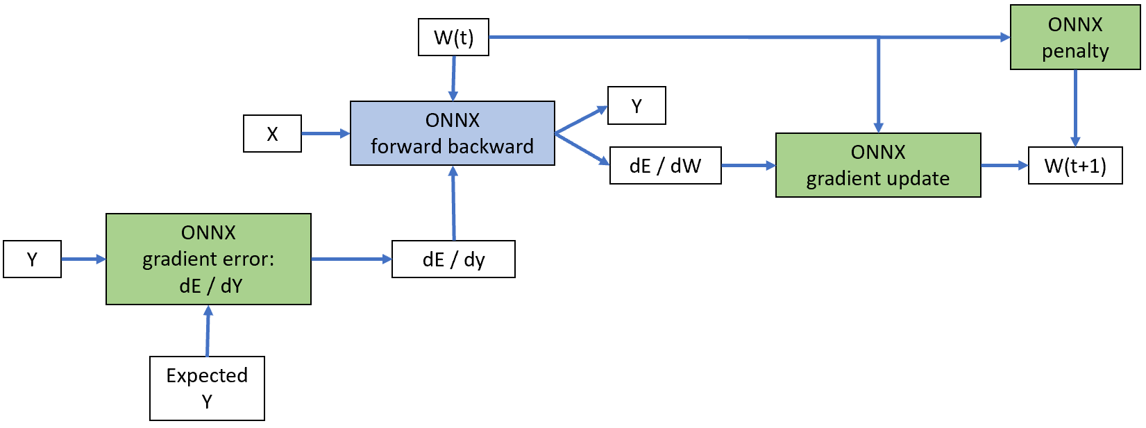
Following graph summarizes how these pieces are gathered altogether. Blue piece is implemented by onnxruntime-training. Green pieces represents the three ONNX graphs needed to compute the loss and its gradient, the regularization, the weight update.
The design seems over complicated
compare to what pytorch does. The main reason is torch.Tensor
supports matrix operations and class OrtValue does not.
They can only be manipulated through ONNX graph and InferenceSession.
These three attributes hide ONNX graph and InferenceSession to compute
loss, regularization and their gradient, and to update the weights accordingly.
These three classes all implement method build_onnx_function which
creates the ONNX graph based on the argument the classes were
initialized with.
Training can then happen this way:
train_session.fit(X_train, y_train, w_train)
Coefficients can be retrieved like the following:
state_tensors = train_session.get_state()
And train losses:
losses = train_session.train_losses_
Method save_onnx_graph
exports all graphs used by a model. It can be saved on disk
or just serialized in memory.
Next examples show that in practice.
Cache#
Base class BaseLearningOnnx implements
methods _bind_input_ortvalue
and _bind_output_ortvalue
used by the three components mentioned above. They cache the binded pointers
(the value returns by c_ortvalue.data_ptr() and do not bind again
if the method is called again with a different OrtValue but a same pointer
returned by data_ptr().
Binary classification#
Probabilities are computed from raw scores with a function such as the
sigmoid function.
A binary function produces two probilities: 
 where s is the raw score. The associated loss
function is usually the log loss:
where s is the raw score. The associated loss
function is usually the log loss:  where y is the expected class (0 or 1),
s=s(X) is the raw score, p(s) is the probability.
We could compute the gradient of the loss
against the probability and let onnxruntime-training handle the
computation of the gradient from the probability to the input.
However, the gradient of the loss against the raw score can easily be
expressed as
where y is the expected class (0 or 1),
s=s(X) is the raw score, p(s) is the probability.
We could compute the gradient of the loss
against the probability and let onnxruntime-training handle the
computation of the gradient from the probability to the input.
However, the gradient of the loss against the raw score can easily be
expressed as  . The second
option is implemented in example Benchmark, comparison sklearn - forward-backward - classification.
. The second
option is implemented in example Benchmark, comparison sklearn - forward-backward - classification.
Examples#
This example assumes the loss function is not part of the graph to train but the gradient of the loss against the graph output is provided. It does not take care to the weight. This part must be separatly implemented as well. Next examples introduce how this is done with ONNX and onnxruntime-training.
- Train a linear regression with forward backward
- Forward backward on a neural network on GPU
- Forward backward on a neural network on GPU (Nesterov) and penalty
- Benchmark, comparison scikit-learn - forward-backward
- Benchmark, comparison sklearn - forward-backward - classification
- Compares numpy to onnxruntime on simple functions