Jeu de données avec des catégories

Links: notebook, html, PDF, python, slides, GitHub

Le jeu de données Adult Data Set ne contient presque que des catégories. Ce notebook explore différentes moyens de les traiter.

%matplotlib inline

from jyquickhelper import add_notebook_menu
add_notebook_menu()

import fiona

données

from papierstat.datasets import load_adult_dataset
train, test = load_adult_dataset(url="copy")
train.head()

	age	workclass	fnlwgt	education	education_num	marital_status	occupation	relationship	race	sex	capital_gain	capital_loss	hours_per_week	native_country	<=50K
0	39	State-gov	77516	Bachelors	13	Never-married	Adm-clerical	Not-in-family	White	Male	2174	0	40	United-States	<=50K
1	50	Self-emp-not-inc	83311	Bachelors	13	Married-civ-spouse	Exec-managerial	Husband	White	Male	0	0	13	United-States	<=50K
2	38	Private	215646	HS-grad	9	Divorced	Handlers-cleaners	Not-in-family	White	Male	0	0	40	United-States	<=50K
3	53	Private	234721	11th	7	Married-civ-spouse	Handlers-cleaners	Husband	Black	Male	0	0	40	United-States	<=50K
4	28	Private	338409	Bachelors	13	Married-civ-spouse	Prof-specialty	Wife	Black	Female	0	0	40	Cuba	<=50K

label = '<=50K'
set(train[label])

{'<=50K', '>50K'}

set(test[label])

{'<=50K', '>50K'}

import numpy
import pandas
X_train = train.drop(label, axis=1)
y_train = train[label] == '>50K'
y_train = pandas.Series(numpy.array([1.0 if y else 0.0 for y in y_train]))
X_test = test.drop(label, axis=1)
y_test = test[label] == '>50K'
y_test = pandas.Series(numpy.array([1.0 if y else 0.0 for y in y_test]))

train.dtypes

age                int64
workclass         object
fnlwgt             int64
education         object
education_num      int64
marital_status    object
occupation        object
relationship      object
race              object
sex               object
capital_gain       int64
capital_loss       int64
hours_per_week     int64
native_country    object
<=50K             object
dtype: object

La variable fnlwgt représente une forme de pondération : le nombre d’individus que chaque observation représente. Elle ne doit pas servir à la prédiction, comme pondération qu’on ignorera : cette pondération n’est pas liée aux données mais à l’échantillon et elle est impossible à construire. Il faut s’en passer.

X_train = X_train.drop(['fnlwgt'], axis=1).copy()
X_test = X_test.drop(['fnlwgt'], axis=1).copy()

catégories

On garde la liste des variables catégorielles.

cat_col = list(_ for _ in X_train.select_dtypes("object").columns)
cat_col

['workclass',
 'education',
 'marital_status',
 'occupation',
 'relationship',
 'race',
 'sex',
 'native_country']

La fonction get_dummies est pratique mais problématique si les modalités de la base d’apprentissage et la base de test sont différentes, ce qui est fréquemment le cas pour les catégories peu fréquentes. Il faudrait regrouper les deux bases, l’appliquer puis sépareer à nouveau. Trop long. On veut utiliser OneHotEncoder et LabelEncoder mais ce n’est pas très pratique parce que OneHotEncoder n’accepte que les colonnes entières et LabelEncoder et peut traiter qu’une colonne à la fois.

from sklearn.pipeline import make_pipeline
from sklearn.preprocessing import LabelEncoder, OneHotEncoder
pipe = make_pipeline(LabelEncoder(), OneHotEncoder())
try:
    pipe.fit(X_train[cat_col[0]], y_train)
except Exception as e:
    print(e)

fit_transform() takes 2 positional arguments but 3 were given

On utilise OneHotEncoder du module category_encoders.

from category_encoders import OneHotEncoder
ce = OneHotEncoder(cols=cat_col, handle_missing='value',
                   drop_invariant=False, handle_unknown='value')
X_train_cat = ce.fit_transform(X_train)
X_train_cat.head()

	age	workclass_1	workclass_2	workclass_3	workclass_4	workclass_5	workclass_6	workclass_7	workclass_8	workclass_9	...	native_country_33	native_country_34	native_country_35	native_country_36	native_country_37	native_country_38	native_country_39	native_country_40	native_country_41	native_country_42
0	39	1	0	0	0	0	0	0	0	0	...	0	0	0	0	0	0	0	0	0	0
1	50	0	1	0	0	0	0	0	0	0	...	0	0	0	0	0	0	0	0	0	0
2	38	0	0	1	0	0	0	0	0	0	...	0	0	0	0	0	0	0	0	0	0
3	53	0	0	1	0	0	0	0	0	0	...	0	0	0	0	0	0	0	0	0	0
4	28	0	0	1	0	0	0	0	0	0	...	0	0	0	0	0	0	0	0	0	0

5 rows × 107 columns

C’est assez compliqué à lire. On renomme les colonnes avec les noms des catégories originaux. Il y a probablement mieux mais ce code fonctionne.

def rename_columns(df, ce):
    rev_mapping = {r['col']: r['mapping'] for r in ce.category_mapping}
    cols = []
    for c in df.columns:
        if '_' not in c:
            cols.append(c)
            continue
        spl = c.split('_')
        col = "_".join(spl[:-1])
        try:
            nb = int(spl[-1])
            mapping  = rev_mapping[col]
            cols.append(str(col) + "__" + str(mapping.index[nb]))
        except ValueError:
            cols.append(c)
    df.columns = cols + list(df.columns)[len(cols):]

rename_columns(X_train_cat, ce)
X_train_cat.head()

	age	workclass__Self-emp-not-inc	workclass__Private	workclass__Federal-gov	workclass__Local-gov	workclass__?	workclass__Self-emp-inc	workclass__Without-pay	workclass__Never-worked	workclass__nan	...	native_country__Scotland	native_country__Trinadad&Tobago	native_country__Greece	native_country__Nicaragua	native_country__Vietnam	native_country__Hong	native_country__Ireland	native_country__Hungary	native_country__Holand-Netherlands	native_country__nan
0	39	1	0	0	0	0	0	0	0	0	...	0	0	0	0	0	0	0	0	0	0
1	50	0	1	0	0	0	0	0	0	0	...	0	0	0	0	0	0	0	0	0	0
2	38	0	0	1	0	0	0	0	0	0	...	0	0	0	0	0	0	0	0	0	0
3	53	0	0	1	0	0	0	0	0	0	...	0	0	0	0	0	0	0	0	0	0
4	28	0	0	1	0	0	0	0	0	0	...	0	0	0	0	0	0	0	0	0	0

5 rows × 107 columns

C’est plus clair. Une dernière remarque sur le paramètre handle_missing et handle_unknown. Le premier définit la façon de gérer les valeurs manquantes, le premier la façon dont le modèle doit gérer les catégories nouvelles, c’est-à-dire les catégories non vues dans la base d’apprentissage.

premier jet

On construit un pipeline.

from sklearn.linear_model import LogisticRegression
pipe = make_pipeline(
            OneHotEncoder(cols=cat_col, handle_missing='value',
                          drop_invariant=False, handle_unknown='value'),
            LogisticRegression())
pipe.fit(X_train, y_train)

C:xavierdupre__home_github_forkscikit-learnsklearnlinear_model_logistic.py:764: ConvergenceWarning: lbfgs failed to converge (status=1):
STOP: TOTAL NO. of ITERATIONS REACHED LIMIT.
Increase the number of iterations (max_iter) or scale the data as shown in:
    https://scikit-learn.org/stable/modules/preprocessing.html
Please also refer to the documentation for alternative solver options:
    https://scikit-learn.org/stable/modules/linear_model.html#logistic-regression
  extra_warning_msg=_LOGISTIC_SOLVER_CONVERGENCE_MSG)

Pipeline(memory=None,
         steps=[('onehotencoder',
                 OneHotEncoder(cols=['workclass', 'education', 'marital_status',
                                     'occupation', 'relationship', 'race',
                                     'sex', 'native_country'],
                               drop_invariant=False, handle_missing='value',
                               handle_unknown='value', return_df=True,
                               use_cat_names=False, verbose=0)),
                ('logisticregression',
                 LogisticRegression(C=1.0, class_weight=None, dual=False,
                                    fit_intercept=True, intercept_scaling=1,
                                    l1_ratio=None, max_iter=100,
                                    multi_class='auto', n_jobs=None,
                                    penalty='l2', random_state=None,
                                    solver='lbfgs', tol=0.0001, verbose=0,
                                    warm_start=False))],
         verbose=False)

pipe.score(X_test, y_test)

0.8426386585590566

On essaye avec une RandomForest.

from sklearn.ensemble import RandomForestClassifier
pipe2 = make_pipeline(ce, RandomForestClassifier(n_estimators=100))
pipe2.fit(X_train, y_train)

Pipeline(memory=None,
         steps=[('onehotencoder',
                 OneHotEncoder(cols=['workclass', 'education', 'marital_status',
                                     'occupation', 'relationship', 'race',
                                     'sex', 'native_country'],
                               drop_invariant=False, handle_missing='value',
                               handle_unknown='value', return_df=True,
                               use_cat_names=False, verbose=0)),
                ('randomforestclassifier',
                 RandomForestClassifier(bootstrap=True, ccp_alpha=0.0,
                                        class_weight=None, criterion='gini',
                                        max_depth=None, max_features='auto',
                                        max_leaf_nodes=None, max_samples=None,
                                        min_impurity_decrease=0.0,
                                        min_impurity_split=None,
                                        min_samples_leaf=1, min_samples_split=2,
                                        min_weight_fraction_leaf=0.0,
                                        n_estimators=100, n_jobs=None,
                                        oob_score=False, random_state=None,
                                        verbose=0, warm_start=False))],
         verbose=False)

pipe2.score(X_test, y_test)

0.8448498249493275

pipe2.steps[-1][-1].feature_importances_[:5]

array([0.22779679, 0.00529596, 0.00965327, 0.01187745, 0.00584904])

On regarde l’importance des features.

import pandas
df = pandas.DataFrame(dict(name=X_train_cat.columns,
                           importance=pipe2.steps[-1][-1].feature_importances_))
df = df.sort_values("importance", ascending=False).reset_index(drop=True)
df = df.set_index('name')
df.head()

	importance
name
age	0.227797
hours_per_week	0.113923
capital_gain	0.110967
marital_status__Divorced	0.067712
education_num	0.064527

import matplotlib.pyplot as plt
fig, ax = plt.subplots(1, 1, figsize=(6, 4))
df[:10].plot.barh(ax=ax)
ax.set_title('Importance des variables - RandomForest');

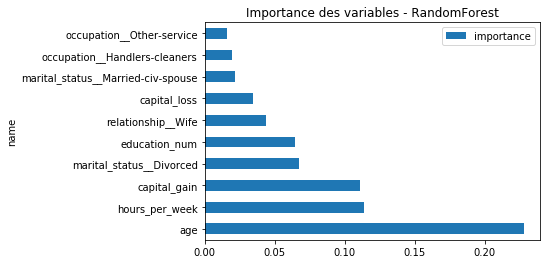
On compare avec XGBoost. L’âge semble la variable plus importante. Cela dit, si ce graphique donne quelques pistes, ce n’est pas la vérité car les variables peuvent être corrélées. Deux variables corrélées sont interchangeables.

from xgboost import XGBClassifier
pipe3 = make_pipeline(ce, XGBClassifier())
pipe3.fit(X_train, y_train)

Pipeline(memory=None,
         steps=[('onehotencoder',
                 OneHotEncoder(cols=['workclass', 'education', 'marital_status',
                                     'occupation', 'relationship', 'race',
                                     'sex', 'native_country'],
                               drop_invariant=False, handle_missing='value',
                               handle_unknown='value', return_df=True,
                               use_cat_names=False, verbose=0)),
                ('xgbclassifier',
                 XGBClassifier(base_score=0.5, booster='gbtree',
                               colsample_bylevel=1, colsample_bynode=1,
                               colsample_bytree=1, gamma=0, learning_rate=0.1,
                               max_delta_step=0, max_depth=3,
                               min_child_weight=1, missing=None,
                               n_estimators=100, n_jobs=1, nthread=None,
                               objective='binary:logistic', random_state=0,
                               reg_alpha=0, reg_lambda=1, scale_pos_weight=1,
                               seed=None, silent=None, subsample=1,
                               verbosity=1))],
         verbose=False)

pipe3.score(X_test, y_test)

0.869172655242307

df = pandas.DataFrame(dict(name=X_train_cat.columns,
                           importance=pipe3.steps[-1][-1].feature_importances_))
df = df.sort_values("importance", ascending=False).reset_index(drop=True)
df = df.set_index('name')
fig, ax = plt.subplots(1, 1, figsize=(6, 4))
df[:10].plot.barh(ax=ax)
ax.set_title('Importance des variables - XGBoost');

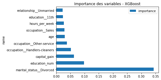
On retrouve presque les mêmes variables mais pas dans le même ordre. On essaye un dernier module catboost.

from catboost import CatBoostClassifier
pipe4 = make_pipeline(ce, CatBoostClassifier(iterations=100, verbose=False))
pipe4.fit(X_train, y_train)

Pipeline(memory=None,
         steps=[('onehotencoder',
                 OneHotEncoder(cols=['workclass', 'education', 'marital_status',
                                     'occupation', 'relationship', 'race',
                                     'sex', 'native_country'],
                               drop_invariant=False, handle_missing='value',
                               handle_unknown='value', return_df=True,
                               use_cat_names=False, verbose=0)),
                ('catboostclassifier',
                 <catboost.core.CatBoostClassifier object at 0x000001E0DF767AC8>)],
         verbose=False)

pipe4.score(X_test, y_test)

0.0

df = pandas.DataFrame(dict(name=X_train_cat.columns,
                           importance=pipe4.steps[-1][-1].feature_importances_))
df = df.sort_values("importance", ascending=False).reset_index(drop=True)
df = df.set_index('name')
fig, ax = plt.subplots(1, 1, figsize=(6, 4))
df[:10].plot.barh(ax=ax)
ax.set_title('Importance des variables - CatBoost');

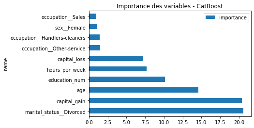
Les modèles sont à peu près d’accord sur la performance mais pas vraiment sur l’ordre des features les plus importantes. Comme ce sont tous des random forests, même apprises différemment, on peut supposer qu’il existe des corrélations entre les variables. Des corrélations au sens du modèle donc pas nécessairement linéaires.

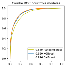
Courbe ROC

from sklearn.metrics import roc_curve
import warnings
if len(pipe2.steps[-1][-1].classes_) != len(pipe3.steps[-1][-1].classes_):
    raise Exception("Mésentente classificatoire pipe2 {0} != pipe3 {1}".format(
                    pipe2.steps[-1][-1].classes_, pipe3.steps[-1][-1].classes_))
if len(pipe2.steps[-1][-1].classes_) != len(pipe4.steps[-1][-1].classes_):
    if not pipe4.steps[-1][-1].classes_:
        # Probably a bug (happens on circleci).
        # Assuming classes are in the same order.
        # See https://github.com/catboost/catboost/blob/master/catboost/python-package/catboost/core.py#L1994
        warnings.warn("pipe4.steps[-1][-1].classes_ is empty.")
        pipe4.steps[-1][-1]._classes = pipe2.steps[-1][-1].classes_
if len(pipe2.steps[-1][-1].classes_) != len(pipe4.steps[-1][-1].classes_):
    print("Mésentente classificatoire pipe2 {0} != pipe4 {1}".format(
                    pipe2.steps[-1][-1].classes_, pipe4.steps[-1][-1].classes_))

index2 = pipe2.steps[-1][-1].classes_[1]
index3 = pipe3.steps[-1][-1].classes_[1]
index4 = pipe4.steps[-1][-1].classes_[1]
fpr2, tpr2, th2 = roc_curve(y_test, pipe2.predict_proba(X_test)[:, 1],
                            pos_label=index2, drop_intermediate=False)
fpr3, tpr3, th3 = roc_curve(y_test, pipe3.predict_proba(X_test)[:, 1],
                            pos_label=index3, drop_intermediate=False)
if len(pipe4.steps[-1][-1].classes_) >= 2:
    fpr4, tpr4, th4 = roc_curve(y_test, pipe4.predict_proba(X_test)[:, 1],
                                pos_label=index4, drop_intermediate=False)
else:
    fpr4 = None

from sklearn.metrics import auc
fig, ax = plt.subplots(1, 1, figsize=(4, 4))
ax.plot(fpr2, tpr2, label='%1.3f RandomForest' % auc(fpr2, tpr2), color='y')
ax.plot(fpr3, tpr3, label='%1.3f XGBoost' % auc(fpr3, tpr3))
if fpr4 is not None:
    ax.plot(fpr4, tpr4, label='%1.3f CatBoost' % auc(fpr4, tpr4))
ax.legend()
ax.set_title('Courbe ROC pour trois modèles');

GridSearch

On cherche à optimiser les hyperparamètres sur la base d’apprentissage. On vérifie d’abord que les données sont bien identiquement distribuées. La validation croisée considère des parties contigües de la base de données. Il arrive que les données ne soient pas tout-à-fait homogènes et qu’il faille les mélanger. On compare les performances avant et après mélange pour vérifier que l’ordre des données n’a pas d’incidence.

from sklearn.model_selection import cross_val_score
cross_val_score(pipe2, X_train, y_train, cv=5)

array([0.84707508, 0.84152334, 0.84259828, 0.85288698, 0.84766585])

from pandas_streaming.df import dataframe_shuffle
from numpy.random import permutation
index = permutation(X_train.index)
X_train_shuffled = X_train.iloc[index, :]
y_train_shuffled = y_train[index]
cross_val_score(pipe2, X_train_shuffled, y_train_shuffled, cv=5)

array([0.84277599, 0.84797297, 0.84659091, 0.84981572, 0.85089066])

L’ordre de la base n’a pas d’incidence.

from sklearn.model_selection import GridSearchCV
param_grid = {'randomforestclassifier__n_estimators':[10, 20, 50],
              'randomforestclassifier__min_samples_leaf': [2, 10]}
cvgrid = GridSearchCV(estimator=pipe2, param_grid=param_grid, verbose=2)
cvgrid.fit(X_train, y_train)

Fitting 5 folds for each of 6 candidates, totalling 30 fits
[CV] randomforestclassifier__min_samples_leaf=2, randomforestclassifier__n_estimators=10

[Parallel(n_jobs=1)]: Using backend SequentialBackend with 1 concurrent workers.

[CV]  randomforestclassifier__min_samples_leaf=2, randomforestclassifier__n_estimators=10, total=   1.2s
[CV] randomforestclassifier__min_samples_leaf=2, randomforestclassifier__n_estimators=10

[Parallel(n_jobs=1)]: Done   1 out of   1 | elapsed:    1.1s remaining:    0.0s

[CV]  randomforestclassifier__min_samples_leaf=2, randomforestclassifier__n_estimators=10, total=   1.2s
[CV] randomforestclassifier__min_samples_leaf=2, randomforestclassifier__n_estimators=10
[CV]  randomforestclassifier__min_samples_leaf=2, randomforestclassifier__n_estimators=10, total=   1.2s
[CV] randomforestclassifier__min_samples_leaf=2, randomforestclassifier__n_estimators=10
[CV]  randomforestclassifier__min_samples_leaf=2, randomforestclassifier__n_estimators=10, total=   1.2s
[CV] randomforestclassifier__min_samples_leaf=2, randomforestclassifier__n_estimators=10
[CV]  randomforestclassifier__min_samples_leaf=2, randomforestclassifier__n_estimators=10, total=   1.2s
[CV] randomforestclassifier__min_samples_leaf=2, randomforestclassifier__n_estimators=20
[CV]  randomforestclassifier__min_samples_leaf=2, randomforestclassifier__n_estimators=20, total=   1.6s
[CV] randomforestclassifier__min_samples_leaf=2, randomforestclassifier__n_estimators=20
[CV]  randomforestclassifier__min_samples_leaf=2, randomforestclassifier__n_estimators=20, total=   1.6s
[CV] randomforestclassifier__min_samples_leaf=2, randomforestclassifier__n_estimators=20
[CV]  randomforestclassifier__min_samples_leaf=2, randomforestclassifier__n_estimators=20, total=   1.6s
[CV] randomforestclassifier__min_samples_leaf=2, randomforestclassifier__n_estimators=20
[CV]  randomforestclassifier__min_samples_leaf=2, randomforestclassifier__n_estimators=20, total=   1.5s
[CV] randomforestclassifier__min_samples_leaf=2, randomforestclassifier__n_estimators=20
[CV]  randomforestclassifier__min_samples_leaf=2, randomforestclassifier__n_estimators=20, total=   1.6s
[CV] randomforestclassifier__min_samples_leaf=2, randomforestclassifier__n_estimators=50
[CV]  randomforestclassifier__min_samples_leaf=2, randomforestclassifier__n_estimators=50, total=   2.6s
[CV] randomforestclassifier__min_samples_leaf=2, randomforestclassifier__n_estimators=50
[CV]  randomforestclassifier__min_samples_leaf=2, randomforestclassifier__n_estimators=50, total=   3.2s
[CV] randomforestclassifier__min_samples_leaf=2, randomforestclassifier__n_estimators=50
[CV]  randomforestclassifier__min_samples_leaf=2, randomforestclassifier__n_estimators=50, total=   3.4s
[CV] randomforestclassifier__min_samples_leaf=2, randomforestclassifier__n_estimators=50
[CV]  randomforestclassifier__min_samples_leaf=2, randomforestclassifier__n_estimators=50, total=   3.6s
[CV] randomforestclassifier__min_samples_leaf=2, randomforestclassifier__n_estimators=50
[CV]  randomforestclassifier__min_samples_leaf=2, randomforestclassifier__n_estimators=50, total=   2.8s
[CV] randomforestclassifier__min_samples_leaf=10, randomforestclassifier__n_estimators=10
[CV]  randomforestclassifier__min_samples_leaf=10, randomforestclassifier__n_estimators=10, total=   1.4s
[CV] randomforestclassifier__min_samples_leaf=10, randomforestclassifier__n_estimators=10
[CV]  randomforestclassifier__min_samples_leaf=10, randomforestclassifier__n_estimators=10, total=   1.2s
[CV] randomforestclassifier__min_samples_leaf=10, randomforestclassifier__n_estimators=10
[CV]  randomforestclassifier__min_samples_leaf=10, randomforestclassifier__n_estimators=10, total=   1.1s
[CV] randomforestclassifier__min_samples_leaf=10, randomforestclassifier__n_estimators=10
[CV]  randomforestclassifier__min_samples_leaf=10, randomforestclassifier__n_estimators=10, total=   1.1s
[CV] randomforestclassifier__min_samples_leaf=10, randomforestclassifier__n_estimators=10
[CV]  randomforestclassifier__min_samples_leaf=10, randomforestclassifier__n_estimators=10, total=   1.1s
[CV] randomforestclassifier__min_samples_leaf=10, randomforestclassifier__n_estimators=20
[CV]  randomforestclassifier__min_samples_leaf=10, randomforestclassifier__n_estimators=20, total=   1.4s
[CV] randomforestclassifier__min_samples_leaf=10, randomforestclassifier__n_estimators=20
[CV]  randomforestclassifier__min_samples_leaf=10, randomforestclassifier__n_estimators=20, total=   1.4s
[CV] randomforestclassifier__min_samples_leaf=10, randomforestclassifier__n_estimators=20
[CV]  randomforestclassifier__min_samples_leaf=10, randomforestclassifier__n_estimators=20, total=   1.5s
[CV] randomforestclassifier__min_samples_leaf=10, randomforestclassifier__n_estimators=20
[CV]  randomforestclassifier__min_samples_leaf=10, randomforestclassifier__n_estimators=20, total=   1.6s
[CV] randomforestclassifier__min_samples_leaf=10, randomforestclassifier__n_estimators=20
[CV]  randomforestclassifier__min_samples_leaf=10, randomforestclassifier__n_estimators=20, total=   1.6s
[CV] randomforestclassifier__min_samples_leaf=10, randomforestclassifier__n_estimators=50
[CV]  randomforestclassifier__min_samples_leaf=10, randomforestclassifier__n_estimators=50, total=   2.4s
[CV] randomforestclassifier__min_samples_leaf=10, randomforestclassifier__n_estimators=50
[CV]  randomforestclassifier__min_samples_leaf=10, randomforestclassifier__n_estimators=50, total=   2.8s
[CV] randomforestclassifier__min_samples_leaf=10, randomforestclassifier__n_estimators=50
[CV]  randomforestclassifier__min_samples_leaf=10, randomforestclassifier__n_estimators=50, total=   2.9s
[CV] randomforestclassifier__min_samples_leaf=10, randomforestclassifier__n_estimators=50
[CV]  randomforestclassifier__min_samples_leaf=10, randomforestclassifier__n_estimators=50, total=   3.9s
[CV] randomforestclassifier__min_samples_leaf=10, randomforestclassifier__n_estimators=50
[CV]  randomforestclassifier__min_samples_leaf=10, randomforestclassifier__n_estimators=50, total=   3.1s

[Parallel(n_jobs=1)]: Done  30 out of  30 | elapsed:   58.3s finished

GridSearchCV(cv=None, error_score=nan,
             estimator=Pipeline(memory=None,
                                steps=[('onehotencoder',
                                        OneHotEncoder(cols=['workclass',
                                                            'education',
                                                            'marital_status',
                                                            'occupation',
                                                            'relationship',
                                                            'race', 'sex',
                                                            'native_country'],
                                                      drop_invariant=False,
                                                      handle_missing='value',
                                                      handle_unknown='value',
                                                      return_df=True,
                                                      use_cat_names=False,
                                                      verbose=0)),
                                       ('randomforestclassifier...
                                                               min_weight_fraction_leaf=0.0,
                                                               n_estimators=100,
                                                               n_jobs=None,
                                                               oob_score=False,
                                                               random_state=None,
                                                               verbose=0,
                                                               warm_start=False))],
                                verbose=False),
             iid='deprecated', n_jobs=None,
             param_grid={'randomforestclassifier__min_samples_leaf': [2, 10],
                         'randomforestclassifier__n_estimators': [10, 20, 50]},
             pre_dispatch='2*n_jobs', refit=True, return_train_score=False,
             scoring=None, verbose=2)

import pandas
df = pandas.DataFrame(cvgrid.cv_results_['params'])
df['mean_fit_time'] = cvgrid.cv_results_['mean_fit_time']
df['mean_test_score'] = cvgrid.cv_results_['mean_test_score']
df.sort_values('mean_test_score')

	randomforestclassifier__min_samples_leaf	randomforestclassifier__n_estimators	mean_fit_time	mean_test_score
3	10	10	1.069937	0.857437
4	10	20	1.351183	0.858635
5	10	50	2.862142	0.859034
0	2	10	1.094900	0.861092
1	2	20	1.456303	0.863641
2	2	50	2.944120	0.863764

Il faudrait continuer à explorer les hyperparamètres et confirmer sur la base de test. A priori, cela marche mieux avec plus d’arbres.

Features polynômiales

On essaye même si cela a peu de chance d’aboutir compte tenu des variables, principalement catégorielles, et du fait qu’on utilise une forêt aléatoire.

from sklearn.preprocessing import PolynomialFeatures
pipe5 = make_pipeline(ce, PolynomialFeatures(), RandomForestClassifier())
pipe5.fit(X_train, y_train)

Pipeline(memory=None,
         steps=[('onehotencoder',
                 OneHotEncoder(cols=['workclass', 'education', 'marital_status',
                                     'occupation', 'relationship', 'race',
                                     'sex', 'native_country'],
                               drop_invariant=False, handle_missing='value',
                               handle_unknown='value', return_df=True,
                               use_cat_names=False, verbose=0)),
                ('polynomialfeatures',
                 PolynomialFeatures(degree=2, include_bias=True,
                                    int...
                 RandomForestClassifier(bootstrap=True, ccp_alpha=0.0,
                                        class_weight=None, criterion='gini',
                                        max_depth=None, max_features='auto',
                                        max_leaf_nodes=None, max_samples=None,
                                        min_impurity_decrease=0.0,
                                        min_impurity_split=None,
                                        min_samples_leaf=1, min_samples_split=2,
                                        min_weight_fraction_leaf=0.0,
                                        n_estimators=100, n_jobs=None,
                                        oob_score=False, random_state=None,
                                        verbose=0, warm_start=False))],
         verbose=False)

pipe5.score(X_test, y_test)

0.8463853571647934

Ca n’améliore pas.

Interprétation

On souhaite en savoir plus sur les variables.

conc = pandas.concat([X_train_cat, pandas.Series(y_train)], axis=1)
conc.head()

	age	workclass__Self-emp-not-inc	workclass__Private	workclass__Federal-gov	workclass__Local-gov	workclass__?	workclass__Self-emp-inc	workclass__Without-pay	workclass__Never-worked	workclass__nan	...	native_country__Trinadad&Tobago	native_country__Greece	native_country__Nicaragua	native_country__Vietnam	native_country__Hong	native_country__Ireland	native_country__Hungary	native_country__Holand-Netherlands	native_country__nan	0
0	39	1	0	0	0	0	0	0	0	0	...	0	0	0	0	0	0	0	0	0	0.0
1	50	0	1	0	0	0	0	0	0	0	...	0	0	0	0	0	0	0	0	0	0.0
2	38	0	0	1	0	0	0	0	0	0	...	0	0	0	0	0	0	0	0	0	0.0
3	53	0	0	1	0	0	0	0	0	0	...	0	0	0	0	0	0	0	0	0	0.0
4	28	0	0	1	0	0	0	0	0	0	...	0	0	0	0	0	0	0	0	0	0.0

5 rows × 108 columns

corr = conc.corr()

from seaborn import clustermap

clustermap(corr, center=0, cmap="vlag", linewidths=.75, figsize=(15, 15));

c:python372_x64libsite-packagesstatsmodelstools_testing.py:19: FutureWarning: pandas.util.testing is deprecated. Use the functions in the public API at pandas.testing instead.
  import pandas.util.testing as tm
c:python372_x64libsite-packagesseabornmatrix.py:624: UserWarning: Clustering large matrix with scipy. Installing fastcluster may give better performance.
  warnings.warn(msg)

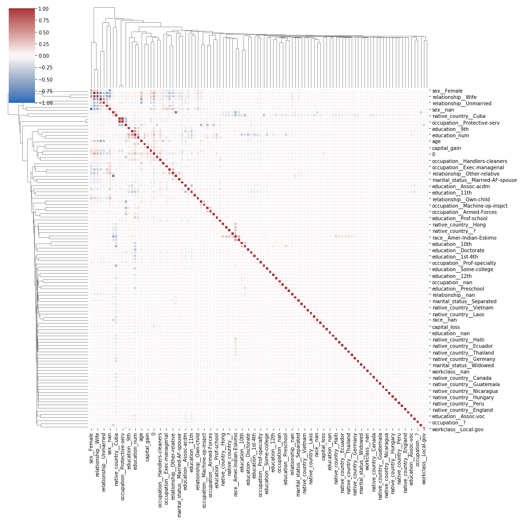
Ce n’est pas facile à voir. Il faudrait essayer avec bokeh ou essayer de procéder autrement.

ACM

Ce qui suit n’est pas tout-à-fait une ACM mais cela s’en inspire. On considère les variables comme des observations et on les projette sur des plans définis par les axes d’une ACP. On normalise également car on mélange variables continues et variables binaires d’ordre de grandeur différents. Les calculs sont plus précis lorsque les matrices ont des coefficients de même ordre. Le dernier exercice de cet examen Programmation ENSAE 2006 achèvera de vous convaincre.

from sklearn.preprocessing import StandardScaler
import pandas
rows_cat = pandas.DataFrame(StandardScaler().fit_transform(X_train_cat))
rows_cat.columns = X_train_cat.columns
rows_cat = rows_cat.T
rows_cat.head(n=2)

	0	1	2	3	4	5	6	7	8	9	...	32551	32552	32553	32554	32555	32556	32557	32558	32559	32560
age	0.030671	0.837109	-0.042642	1.057047	-0.775768	-0.115955	0.763796	0.983734	-0.555830	0.250608	...	-0.482518	0.323921	-0.482518	1.057047	-1.215643	-0.849080	0.103983	1.423610	-1.215643	0.983734
workclass__Self-emp-not-inc	4.907700	-0.203761	-0.203761	-0.203761	-0.203761	-0.203761	-0.203761	-0.203761	-0.203761	-0.203761	...	-0.203761	-0.203761	-0.203761	-0.203761	-0.203761	-0.203761	-0.203761	-0.203761	-0.203761	-0.203761

2 rows × 32561 columns

from sklearn.decomposition import PCA
pca = PCA(n_components=3)
pca.fit(rows_cat)

PCA(copy=True, iterated_power='auto', n_components=3, random_state=None,
    svd_solver='auto', tol=0.0, whiten=False)

import pandas
tr = pandas.DataFrame(pca.transform(rows_cat))
tr.columns = ['axe1', 'axe2', 'axe3']
tr.index = rows_cat.index
tr.sort_values('axe1').head(n=2)

	axe1	axe2	axe3
sex__nan	-129.499567	60.907917	29.421935
marital_status__Married-civ-spouse	-106.135296	-11.383937	-54.355587

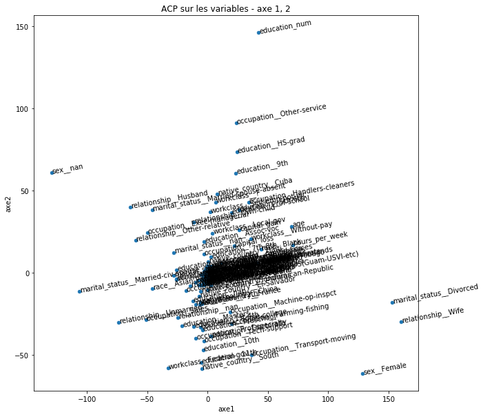
ax = tr.plot(x='axe1', y='axe2', kind='scatter', figsize=(10, 10))
for t, (x, y, z) in tr.iterrows():
    ax.text(x, y, t, fontsize=10, rotation=10)
ax.set_title("ACP sur les variables - axe 1, 2");

ax = tr.plot(x='axe1', y='axe3', kind='scatter', figsize=(10, 10))
for t, (x, y, z) in tr.iterrows():
    ax.text(x, z, t, fontsize=10, rotation=10)
ax.set_title("ACP sur les variables - axe 1, 3");

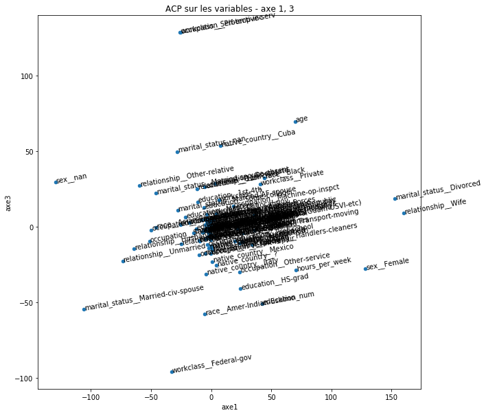
On voit quelques variables à supprimer car très corrélées comme la relation ou la situation maritale. On voit aussi que les deux genres homme/femme sont opposés. On voit aussi que certaines catégories sont très proches comme Prof, Masters ou diplômés. Il est probable que le modèle de prédiction ne pâtisse pas du regroupement de ces trois catégories. On utilise bokeh pour pouvoir zoomer.

import bokeh, bokeh.io as bio
bio.output_notebook()

Loading BokehJS ...

from bokeh.plotting import figure, show
p = figure(title="ACP sur les variables - axe 1, 2")
p.circle(tr["axe1"], tr["axe2"])
p.text(tr["axe1"], tr["axe2"], tr.index,
       text_font_size="8pt", text_baseline="middle", angle=0.1)
show(p)

Analyse d’erreur

On recherche les erreurs les plus flagrantes, celles dont le score est élevé.

pred = pipe.predict(X_test)
proba = pipe.predict_proba(X_test)
pred2 = pipe2.predict(X_test)
proba2 = pipe2.predict_proba(X_test)
pred3 = pipe3.predict(X_test)
proba3 = pipe3.predict_proba(X_test)
pred4 = pipe4.predict(X_test)
proba4 = pipe4.predict_proba(X_test)

data = pandas.concat([
            pandas.DataFrame(y_test.astype(float).values, columns=['y_test']),
            pandas.DataFrame(pred, columns=['pred1']),
            pandas.DataFrame(proba[:,1], columns=['P1(>=50K)']),
            pandas.DataFrame(pred2, columns=['pred2']),
            pandas.DataFrame(proba2[:,1], columns=['P2(>=50K)']),
            pandas.DataFrame(pred3, columns=['pred3']),
            pandas.DataFrame(proba3[:,1], columns=['P3(>=50K)']),
            pandas.DataFrame(pred4, columns=['pred4']),
            pandas.DataFrame(proba4[:,1], columns=['P4(>=50K)']),
            X_test,
            ], axis=1)
data.head()

	y_test	pred1	P1(>=50K)	pred2	P2(>=50K)	pred3	P3(>=50K)	pred4	P4(>=50K)	age	...	education_num	marital_status	occupation	relationship	race	sex	capital_gain	capital_loss	hours_per_week	native_country
0	0.0	0.0	0.010831	0.0	0.000000	0.0	0.007642	0.0	0.000384	25	...	7	Never-married	Machine-op-inspct	Own-child	Black	Male	0	0	40	United-States
1	0.0	0.0	0.179896	0.0	0.030000	0.0	0.203497	0.0	0.207168	38	...	9	Married-civ-spouse	Farming-fishing	Husband	White	Male	0	0	50	United-States
2	1.0	1.0	0.526712	1.0	0.526667	0.0	0.277167	0.0	0.471523	28	...	12	Married-civ-spouse	Protective-serv	Husband	White	Male	0	0	40	United-States
3	1.0	1.0	0.789027	1.0	0.930000	1.0	0.984138	1.0	0.987516	44	...	10	Married-civ-spouse	Machine-op-inspct	Husband	Black	Male	7688	0	40	United-States
4	0.0	0.0	0.009680	0.0	0.000000	0.0	0.002210	0.0	0.000151	18	...	10	Never-married	?	Own-child	White	Female	0	0	30	United-States

5 rows × 22 columns

data[data.y_test != data.pred4].sort_values('P4(>=50K)', ascending=False).head().T

	3605	2926	13783	2247	13128
y_test	0	0	0	0	0
pred1	1	1	1	1	1
P1(>=50K)	1	0.793878	0.764859	0.788413	0.832539
pred2	1	1	1	1	1
P2(>=50K)	0.74	0.74	0.937333	0.94	0.65
pred3	1	1	1	1	1
P3(>=50K)	0.972606	0.900088	0.933867	0.796695	0.913922
pred4	1	1	1	1	1
P4(>=50K)	0.998917	0.989239	0.980988	0.944513	0.931411
age	36	65	51	55	48
workclass	Self-emp-not-inc	Self-emp-not-inc	Private	Self-emp-inc	Local-gov
education	HS-grad	Masters	Some-college	Prof-school	Bachelors
education_num	9	14	10	15	13
marital_status	Married-civ-spouse	Married-spouse-absent	Married-civ-spouse	Married-civ-spouse	Separated
occupation	Exec-managerial	Prof-specialty	Exec-managerial	Prof-specialty	Prof-specialty
relationship	Husband	Not-in-family	Husband	Husband	Unmarried
race	Asian-Pac-Islander	White	White	White	White
sex	Male	Female	Male	Male	Female
capital_gain	41310	7978	0	0	7443
capital_loss	0	0	1902	0	0
hours_per_week	90	40	40	55	45
native_country	South	United-States	United-States	United-States	United-States

Tous les modèles font l’erreur sur ces cinq exemples. Le modèle a toutes les raisons de décider que les personnes gagnent plus de 50k par an, beaucoup d’études, plutôt âge ou travaillant beaucoup.

wrong_study = data[data.y_test != data.pred4].sort_values('P4(>=50K)', ascending=True).head(n=3).T
wrong_study

	10408	5953	3059
y_test	1	1	1
pred1	0	0	0
P1(>=50K)	0.0146811	0.00972505	0.0145646
pred2	0	0	0
P2(>=50K)	0	0	0
pred3	0	0	0
P3(>=50K)	0.00288558	0.00299048	0.00561586
pred4	0	0	0
P4(>=50K)	0.000149386	0.000395875	0.000863302
age	22	20	22
workclass	?	Private	Private
education	Some-college	12th	Some-college
education_num	10	8	10
marital_status	Never-married	Never-married	Never-married
occupation	?	Other-service	Sales
relationship	Own-child	Own-child	Not-in-family
race	White	Black	White
sex	Male	Male	Male
capital_gain	0	0	0
capital_loss	0	0	0
hours_per_week	15	35	25
native_country	?	United-States	United-States

Ceux-ci sont probablement étudiants et déjà aisés. Il faudrait avoir quelques informations sur les parents pour confirmer. On recherche les plus proches voisins dans la base pour voir ce que le modèle répond. Il faut néanmoins appliquer cela sur la base une fois les catégories transformées.

from sklearn.neighbors import NearestNeighbors
knn = NearestNeighbors()
knn.fit(X_train_cat)

NearestNeighbors(algorithm='auto', leaf_size=30, metric='minkowski',
                 metric_params=None, n_jobs=None, n_neighbors=5, p=2,
                 radius=1.0)

X_test_cat = pipe2.steps[0][-1].transform(X_test)
X_test_cat.columns = X_train_cat.columns

wrong = data[data.y_test != data.pred4].sort_values('P4(>=50K)', ascending=True).head()
wrong.head(n=2)

	y_test	pred1	P1(>=50K)	pred2	P2(>=50K)	pred3	P3(>=50K)	pred4	P4(>=50K)	age	...	education_num	marital_status	occupation	relationship	race	sex	capital_gain	capital_loss	hours_per_week	native_country
10408	1.0	0.0	0.014681	0.0	0.0	0.0	0.002886	0.0	0.000149	22	...	10	Never-married	?	Own-child	White	Male	0	0	15	?
5953	1.0	0.0	0.009725	0.0	0.0	0.0	0.002990	0.0	0.000396	20	...	8	Never-married	Other-service	Own-child	Black	Male	0	0	35	United-States

2 rows × 22 columns

wrong_cat = X_test_cat.iloc[wrong.index, :]
wrong_cat.head()

	age	workclass__Self-emp-not-inc	workclass__Private	workclass__Federal-gov	workclass__Local-gov	workclass__?	workclass__Self-emp-inc	workclass__Without-pay	workclass__Never-worked	workclass__nan	...	native_country__Scotland	native_country__Trinadad&Tobago	native_country__Greece	native_country__Nicaragua	native_country__Vietnam	native_country__Hong	native_country__Ireland	native_country__Hungary	native_country__Holand-Netherlands	native_country__nan
10408	22	0	0	0	0	0	1	0	0	0	...	0	0	0	0	0	0	0	0	0	0
5953	20	0	0	1	0	0	0	0	0	0	...	0	0	0	0	0	0	0	0	0	0
3059	22	0	0	1	0	0	0	0	0	0	...	0	0	0	0	0	0	0	0	0	0
11821	24	0	0	1	0	0	0	0	0	0	...	0	0	0	0	0	0	0	0	0	0
12808	67	0	0	1	0	0	0	0	0	0	...	0	0	0	0	0	0	0	0	0	0

5 rows × 107 columns

dist, index = knn.kneighbors(wrong_cat)
dist

array([[2.        , 2.        , 2.23606798, 2.44948974, 2.44948974],
       [1.41421356, 1.41421356, 2.23606798, 2.23606798, 2.23606798],
       [1.        , 1.41421356, 1.41421356, 1.73205081, 1.73205081],
       [1.41421356, 1.73205081, 1.73205081, 1.73205081, 2.        ],
       [2.64575131, 3.31662479, 3.46410162, 3.46410162, 3.74165739]])

index

array([[18056, 18362,  8757, 13177,   314],
       [24878, 30060, 27902,  8008, 23771],
       [  920, 31176,  5206,  7415, 15308],
       [17303, 18592,  2019, 20325,  7542],
       [  346, 14421,  8214, 11050, 18902]], dtype=int64)

train_nn = pandas.concat([X_train, y_train], axis=1).iloc[[24878, 18056, 920], :].T
train_nn.columns = ['TR-' + str(_) for _ in train_nn.columns]
train_nn

	TR-24878	TR-18056	TR-920
age	20	21	23
workclass	Private	?	Private
education	12th	Some-college	Some-college
education_num	8	10	10
marital_status	Never-married	Never-married	Never-married
occupation	Other-service	?	Sales
relationship	Own-child	Own-child	Not-in-family
race	White	White	White
sex	Male	Male	Male
capital_gain	0	0	0
capital_loss	0	0	0
hours_per_week	35	16	25
native_country	United-States	United-States	United-States
0	0	0	0

Il faut comparer la première colonne avec la quatrième, la seconde avec la ciinquième et la troisème avec la sixième. Ces exemples sont voisins. On voit que les exemples sont très proches. Il n’y a qu’une seule valeur qui change à chaque fois et il est difficile d’expliquer les erreurs.

pandas.concat([train_nn, wrong_study], axis=1, sort=True)

	TR-24878	TR-18056	TR-920	10408	5953	3059
age	20	21	23	22	20	22
capital_gain	0	0	0	0	0	0
capital_loss	0	0	0	0	0	0
education	12th	Some-college	Some-college	Some-college	12th	Some-college
education_num	8	10	10	10	8	10
hours_per_week	35	16	25	15	35	25
marital_status	Never-married	Never-married	Never-married	Never-married	Never-married	Never-married
native_country	United-States	United-States	United-States	?	United-States	United-States
occupation	Other-service	?	Sales	?	Other-service	Sales
race	White	White	White	White	Black	White
relationship	Own-child	Own-child	Not-in-family	Own-child	Own-child	Not-in-family
sex	Male	Male	Male	Male	Male	Male
workclass	Private	?	Private	?	Private	Private
0	0	0	0	NaN	NaN	NaN
y_test	NaN	NaN	NaN	1	1	1
pred1	NaN	NaN	NaN	0	0	0
P1(>=50K)	NaN	NaN	NaN	0.0146811	0.00972505	0.0145646
pred2	NaN	NaN	NaN	0	0	0
P2(>=50K)	NaN	NaN	NaN	0	0	0
pred3	NaN	NaN	NaN	0	0	0
P3(>=50K)	NaN	NaN	NaN	0.00288558	0.00299048	0.00561586
pred4	NaN	NaN	NaN	0	0	0
P4(>=50K)	NaN	NaN	NaN	0.000149386	0.000395875	0.000863302

Ethique

Le modèle qu’on a appris est-il éthique ? Il n’y a pas de réponse simples à ce problème car il est difficile de transcrire mathématiquement le caractère éthique d’un modèle. Dans le cas présent, admettons que l’on souhaite vérifier que le modèle ne retourne pas une réponse biaisée en fonction du genre. Une première idée consiste à enlever la variable pour être sûr sur le modèle n’en tienne pas compte mais cela ne garantit que la variable genre n’est une variable corrélée aux autres. Et la corrélation implique ici au sens du modèle ce qui a un sens plus fort si le modèle n’est pas linéaire. On aura tout-à-faire enlevé la variable genre si elle ne peut être prédite à partir des autres.

X_train_sex = train.drop([label, 'sex'], axis=1)
y_train_sex = train['sex'] == 'Male'
X_test_sex = test.drop([label, 'sex'], axis=1)
y_test_sex = test['sex'] == 'Male'

ce_sex = OneHotEncoder(cols=[_ for _ in cat_col if _ != 'sex'],
                       handle_missing='value', drop_invariant=False,
                       handle_unknown='value')
model_sex = make_pipeline(ce_sex, RandomForestClassifier(n_estimators=100))
model_sex.fit(X_train_sex, y_train_sex)

Pipeline(memory=None,
         steps=[('onehotencoder',
                 OneHotEncoder(cols=['workclass', 'education', 'marital_status',
                                     'occupation', 'relationship', 'race',
                                     'native_country'],
                               drop_invariant=False, handle_missing='value',
                               handle_unknown='value', return_df=True,
                               use_cat_names=False, verbose=0)),
                ('randomforestclassifier',
                 RandomForestClassifier(bootstrap=True, ccp_alpha=0.0,
                                        class_weight=None, criterion='gini',
                                        max_depth=None, max_features='auto',
                                        max_leaf_nodes=None, max_samples=None,
                                        min_impurity_decrease=0.0,
                                        min_impurity_split=None,
                                        min_samples_leaf=1, min_samples_split=2,
                                        min_weight_fraction_leaf=0.0,
                                        n_estimators=100, n_jobs=None,
                                        oob_score=False, random_state=None,
                                        verbose=0, warm_start=False))],
         verbose=False)

model_sex.score(X_test_sex, y_test_sex)

0.8368650574289048

Il est possible de prédire le genre en fonction des autres variables à 83% près. Ce n’est pas en enlevant la variable qu’on peut empêcher le modèle d’être biaisé par rapport à cette information. Il n’est pas évident de retirer toute influence de ce paramètre. On peut choisir de la garder en supposant que le modèle la choisira plutôt qu’une autre pour prédire si elle s’avère pertinente. Dans ce cas, on pourrait comparer combien de fois le modèle change de prédiction si on inverse la variable sex. On rappelle la performance du modèle.

pipe2.score(X_test, y_test)

0.8448498249493275

On remplace la variable sex par la prédiction de l’autre modèle.

X_test_modified = X_test.copy()
X_test_modified['sex'] = model_sex.predict(X_test_sex)
X_test_modified['sex'] = X_test_modified['sex'].apply(lambda x: 'Male' if x else 'Female')

pipe2.score(X_test_modified, y_test)

0.843928505620048

Quasiment aucun changement. Inversons la colonne maintenant.

X_test_inv = X_test.copy()
X_test_inv['sex'] = X_test_inv['sex'].apply(lambda x: 'Female' if x == 'Male' else 'Male')

pipe2.score(X_test_inv, y_test)

0.8505005835022419

Encore mieux. Regardons les différences maintenant.

diff1 = X_test['sex'] != X_test_inv['sex']
diff2 = pipe2.predict(X_test) != pipe2.predict(X_test_inv)
diff2.sum(), diff1.sum(), diff2.sum() / diff1.sum()

(1024, 16281, 0.06289539954548247)

La prédiction change dans 5% des cas. On est sûr que pour ces observations et ce modèle, le genre a un impact, cela ne veut rien dire pour les autres. Regardons les cinq premières.

look = X_test.copy()
look['y'] = y_test
look['prediction_sex'] = model_sex.predict(X_test_sex)
look[diff2].head().T

	2	14	17	19	28
age	28	48	43	40	54
workclass	Local-gov	Private	Private	Private	Private
education	Assoc-acdm	HS-grad	HS-grad	Doctorate	HS-grad
education_num	12	9	9	16	9
marital_status	Married-civ-spouse	Married-civ-spouse	Married-civ-spouse	Married-civ-spouse	Married-civ-spouse
occupation	Protective-serv	Machine-op-inspct	Adm-clerical	Prof-specialty	Craft-repair
relationship	Husband	Husband	Wife	Husband	Husband
race	White	White	White	Asian-Pac-Islander	White
sex	Male	Male	Female	Male	Male
capital_gain	0	3103	0	0	0
capital_loss	0	0	0	0	0
hours_per_week	40	48	30	45	35
native_country	United-States	United-States	United-States	?	United-States
y	1	1	0	1	0
prediction_sex	True	True	False	True	True

Il existe visible quelques observations à vérifier où la relation relationship et le genre sex semble être en contradiction ou plutôt ne pas prendre en compte tous les types de relations possibles.

X_train[['sex', 'relationship', 'age']].groupby(['sex', 'relationship'], as_index=False)\
        .count().pivot('sex', 'relationship', 'age')

relationship	Husband	Not-in-family	Other-relative	Own-child	Unmarried	Wife
sex
Female	1	3875	430	2245	2654	1566
Male	13192	4430	551	2823	792	2

Pas de conclusion à ce stade. Il faut poursuivre l’exploration Machine Learning éthique.

Sélection des variables

Il n’y a pas de méthode optimale pour sélectionner les variables. Il existe différentes options comme celles proposées par scikit-learn/feature_selection. Certaines partent des features brutes, d’autres utilisent le modèle qui doit être appris. Mais ce n’est pas toujours évident de faire marcher ces méthodes sur n’importe quel modèle.

from sklearn.feature_selection import RFE
try:
    model = RFE(pipe2)
    model.fit(X_train, y_train)
except Exception as e:
    print(e)

could not convert string to float: 'State-gov'

Dans notre cas, on retire les variables une à une en fonction de l’indicateur feature_importance ce qui n’est pas facile car les variables sont des modalités. Il faut en faire la somme…

def grouped_feature_importance(model, datas, cat_col):
    ce = model.steps[0][-1]
    data_cat = ce.fit_transform(datas)
    rename_columns(data_cat, ce)
    df = pandas.DataFrame(dict(name=data_cat.columns,
                               importance=model.steps[-1][-1].feature_importances_))
    df = df.sort_values("importance", ascending=False).reset_index(drop=True)
    df['raw_var'] = df['name'].apply(lambda x: x.split('__')[0])
    gr = df.groupby('raw_var').sum().sort_values('importance', ascending=True).reset_index(drop=False).copy()
    return gr

fi_global = grouped_feature_importance(pipe2, X_train, cat_col)
fi_global

	raw_var	importance
0	race	0.018372
1	sex	0.019006
2	native_country	0.028188
3	capital_loss	0.034305
4	workclass	0.047340
5	education	0.059821
6	education_num	0.064527
7	relationship	0.083855
8	occupation	0.091443
9	marital_status	0.100458
10	capital_gain	0.110967
11	hours_per_week	0.113923
12	age	0.227797

On fait une boucle.

kept = list(fi_global.raw_var)
res = []
last_removed = None
while len(kept) > 0:
    cat_col_red = set()
    for col in kept:
        if "__" in col:
            col = "__".join(col.split('__')[:-1])
        cat_col_red.add(col)
    cat_col_red = list(cat_col_red)
    X_train_reduced = X_train[cat_col_red]
    X_test_reduced = X_test[cat_col_red]
    ce = OneHotEncoder(cols=cat_col_red, handle_missing='value',
                       drop_invariant=False, handle_unknown='value')
    model = make_pipeline(ce, RandomForestClassifier(n_estimators=5))
    model.fit(X_train_reduced, y_train)
    score = model.score(X_test_reduced, y_test)
    fi = grouped_feature_importance(model, X_train_reduced, cat_col_red)
    r = dict(score=score, features=kept.copy(), nb=len(kept), model=model,
             removed=last_removed, next_remove=fi.iloc[0,0], score_remove=fi.iloc[0,1])
    print(r['nb'], r['score'], last_removed, list(fi.iloc[0,:]), X_train_reduced.shape)
    last_removed = fi.iloc[0,0]
    kept = [_ for _ in kept if _ != last_removed]
    res.append(r)

13 0.8345310484613967 None ['race', 0.017876461431527595] (32561, 13)
12 0.8328112523800749 race ['native_country', 0.030328521242080998] (32561, 12)
11 0.8377863767581843 native_country ['sex', 0.020085260379222935] (32561, 11)
10 0.8366193722744303 sex ['capital_loss', 0.04176572757064676] (32561, 10)
9 0.8286960260426264 capital_loss ['workclass', 0.051745962436835796] (32561, 9)
8 0.8289417111971009 workclass ['education', 0.06708986825516294] (32561, 8)
7 0.8292488176401941 education ['marital_status', 0.10470565098684484] (32561, 7)
6 0.8299858731036177 marital_status ['education_num', 0.12482378792123464] (32561, 6)
5 0.8271604938271605 education_num ['capital_gain', 0.15606710618140648] (32561, 5)
4 0.8043731957496468 capital_gain ['hours_per_week', 0.1952915897722717] (32561, 4)
3 0.8129721761562557 hours_per_week ['age', 0.2703491413657654] (32561, 3)
2 0.8207726798108225 age ['occupation', 0.3492816128792312] (32561, 2)
1 0.7637737239727289 occupation ['relationship', 0.9999999999999999] (32561, 1)

Il faut se rappeler qu’un classifieur constant retournerait environ 76% de bonne classification.

1 - y_test.sum() / len(y_test)

0.7637737239727289