Régression logistique en 2D

Links: notebook, html, PDF, python, slides, GitHub

Prédire la couleur d’un vin à partir de ses composants.

%matplotlib inline

from papierstat.datasets import load_wines_dataset
data = load_wines_dataset()
X = data.drop(['quality', 'color'], axis=1)
y = data['color']

from sklearn.model_selection import train_test_split
X_train, X_test, y_train, y_test = train_test_split(X, y)

from statsmodels.discrete.discrete_model import Logit
model = Logit(y_train == "white", X_train)
res = model.fit()

Optimization terminated successfully.
         Current function value: 0.044575
         Iterations 11

res.summary2()

Model:	Logit	No. Iterations:	11.0000
Dependent Variable:	color	Pseudo R-squared:	0.921
Date:	2018-02-08 00:13	AIC:	456.3398
No. Observations:	4872	BIC:	527.7436
Df Model:	10	Log-Likelihood:	-217.17
Df Residuals:	4861	LL-Null:	-2748.5
Converged:	1.0000	Scale:	1.0000

	Coef.	Std.Err.	z	P>|z|	[0.025	0.975]
fixed_acidity	-1.4449	0.1519	-9.5141	0.0000	-1.7425	-1.1472
volatile_acidity	-12.0133	0.9940	-12.0857	0.0000	-13.9615	-10.0651
citric_acid	0.1218	1.1387	0.1070	0.9148	-2.1101	2.3537
residual_sugar	0.0780	0.0578	1.3484	0.1775	-0.0354	0.1913
chlorides	-33.6942	4.1533	-8.1125	0.0000	-41.8346	-25.5538
free_sulfur_dioxide	-0.0474	0.0149	-3.1804	0.0015	-0.0767	-0.0182
total_sulfur_dioxide	0.0691	0.0055	12.6272	0.0000	0.0584	0.0798
density	45.6528	4.4627	10.2299	0.0000	36.9061	54.3994
pH	-10.0587	1.0255	-9.8086	0.0000	-12.0687	-8.0488
sulphates	-9.1971	1.0697	-8.5980	0.0000	-11.2936	-7.1006
alcohol	0.5328	0.1284	4.1494	0.0000	0.2811	0.7844

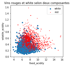
On ne garde que les deux premières.

X_train2 = X_train.iloc[:, :2]

import pandas
df = pandas.DataFrame(X_train2.copy())
df['y'] = y_train

import matplotlib.pyplot as plt
fig, ax = plt.subplots(1, 1, figsize=(4, 4))
df[df.y == "white"].plot(x="fixed_acidity", y="volatile_acidity", ax=ax, kind='scatter', label="white")
df[df.y == "red"].plot(x="fixed_acidity", y="volatile_acidity", ax=ax,
                       kind='scatter', label="red", color="red", s=2)
ax.set_title("Vins rouges et white selon deux composantes");

from sklearn.linear_model import LogisticRegression
model = LogisticRegression()
model.fit(X_train2, y_train == "white")

LogisticRegression(C=1.0, class_weight=None, dual=False, fit_intercept=True,
          intercept_scaling=1, max_iter=100, multi_class='ovr', n_jobs=1,
          penalty='l2', random_state=None, solver='liblinear', tol=0.0001,
          verbose=0, warm_start=False)

model.coef_, model.intercept_

(array([[ -0.92015604, -10.76494765]]), array([11.96976599]))

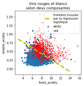
On trace cette droite sur le graphique.

x0 = 3
y0 = -(model.coef_[0,0] * x0 + model.intercept_) / model.coef_[0,1]
x1 = 14
y1 = -(model.coef_[0,0] * x1 + model.intercept_) / model.coef_[0,1]
x0, y0, x1, y1

(3, array([0.85548933]), 14, array([-0.08475829]))

import matplotlib.pyplot as plt
fig, ax = plt.subplots(1, 1, figsize=(4, 4))
df[df.y == "white"].plot(x="fixed_acidity", y="volatile_acidity", ax=ax, kind='scatter', label="white")
df[df.y == "red"].plot(x="fixed_acidity", y="volatile_acidity", ax=ax,
                       kind='scatter', label="red", color="red", s=2)
ax.plot([x0, x1], [y0, y1], 'y--', lw=4, label='frontière trouvée\npar la régression\nlogistique')
ax.legend()
ax.set_title("Vins rouges et blancs\nselon deux composantes");