ROC

An exemple on ROC curve.

Data

from sklearn import datasets
iris = datasets.load_iris()
X = iris.data[:, :2]
y = iris.target

from sklearn.model_selection import train_test_split
X_train, X_test, y_train, y_test = train_test_split(X, y, test_size=0.33)

from sklearn.linear_model import LogisticRegression
clf = LogisticRegression()
clf.fit(X_train, y_train)

LogisticRegression()

In a Jupyter environment, please rerun this cell to show the HTML representation or trust the notebook.
On GitHub, the HTML representation is unable to render, please try loading this page with nbviewer.org.

import numpy
ypred = clf.predict(X_test)
yprob = clf.predict_proba(X_test)
score = numpy.array(list(yprob[i, ypred[i]] for i in range(len(ypred))))

data = numpy.zeros((len(ypred), 2))
data[:, 0] = score.ravel()
data[ypred == y_test, 1] = 1
data[:5]

array([[0.53781077, 1.        ],
       [0.71038639, 1.        ],
       [0.958238  , 1.        ],
       [0.72766728, 1.        ],
       [0.6519351 , 1.        ]])

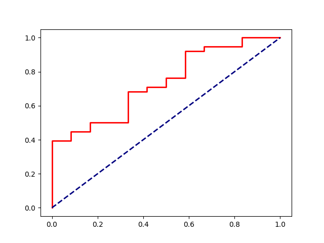
ROC - TPR / FPR

• TPR = True Positive Rate

• FPR = False Positive Rate

You can see as TPR the distribution function of a score for a positive example and the FPR the same for a negative example.

from sklearn import metrics
import matplotlib.pyplot as plt
dec = ypred == y_test
ans = numpy.zeros(len(dec))
ans[dec] = 1
fpr, tpr, thresholds = metrics.roc_curve(ans, score)
plt.figure()
plt.plot(fpr, tpr, lw=2, label='ROC curve', color="red")
plt.plot([0, 1], [0, 1], color='navy', lw=2, linestyle='--')
plt.show()

End

Nothing below.