OnlineNewPopularity (data from UCI)#
Links: notebook, html, PDF, python, slides, GitHub
This notebook suggests a couple of ways to explore the data of a machine learning problem.
from jyquickhelper import add_notebook_menu
add_notebook_menu()
%matplotlib inline
import matplotlib.pyplot as plt
import seaborn
import numpy
import pandas
Download data#
Online News Popularity Data Set
import pyensae.datasource
pyensae.datasource.download_data("OnlineNewsPopularity.zip",
                      url="https://archive.ics.uci.edu/ml/machine-learning-databases/00332/")
['OnlineNewsPopularity/OnlineNewsPopularity.names',
 'OnlineNewsPopularity/OnlineNewsPopularity.csv']
data = pandas.read_csv("OnlineNewsPopularity/OnlineNewsPopularity.csv")
data.columns = [c.strip() for c in data.columns]  # remove spaces around data
data.head()
| url | timedelta | n_tokens_title | n_tokens_content | n_unique_tokens | n_non_stop_words | n_non_stop_unique_tokens | num_hrefs | num_self_hrefs | num_imgs | ... | min_positive_polarity | max_positive_polarity | avg_negative_polarity | min_negative_polarity | max_negative_polarity | title_subjectivity | title_sentiment_polarity | abs_title_subjectivity | abs_title_sentiment_polarity | shares | |
|---|---|---|---|---|---|---|---|---|---|---|---|---|---|---|---|---|---|---|---|---|---|
| 0 | http://mashable.com/2013/01/07/amazon-instant-... | 731.0 | 12.0 | 219.0 | 0.663594 | 1.0 | 0.815385 | 4.0 | 2.0 | 1.0 | ... | 0.100000 | 0.7 | -0.350000 | -0.600 | -0.200000 | 0.500000 | -0.187500 | 0.000000 | 0.187500 | 593 |
| 1 | http://mashable.com/2013/01/07/ap-samsung-spon... | 731.0 | 9.0 | 255.0 | 0.604743 | 1.0 | 0.791946 | 3.0 | 1.0 | 1.0 | ... | 0.033333 | 0.7 | -0.118750 | -0.125 | -0.100000 | 0.000000 | 0.000000 | 0.500000 | 0.000000 | 711 |
| 2 | http://mashable.com/2013/01/07/apple-40-billio... | 731.0 | 9.0 | 211.0 | 0.575130 | 1.0 | 0.663866 | 3.0 | 1.0 | 1.0 | ... | 0.100000 | 1.0 | -0.466667 | -0.800 | -0.133333 | 0.000000 | 0.000000 | 0.500000 | 0.000000 | 1500 |
| 3 | http://mashable.com/2013/01/07/astronaut-notre... | 731.0 | 9.0 | 531.0 | 0.503788 | 1.0 | 0.665635 | 9.0 | 0.0 | 1.0 | ... | 0.136364 | 0.8 | -0.369697 | -0.600 | -0.166667 | 0.000000 | 0.000000 | 0.500000 | 0.000000 | 1200 |
| 4 | http://mashable.com/2013/01/07/att-u-verse-apps/ | 731.0 | 13.0 | 1072.0 | 0.415646 | 1.0 | 0.540890 | 19.0 | 19.0 | 20.0 | ... | 0.033333 | 1.0 | -0.220192 | -0.500 | -0.050000 | 0.454545 | 0.136364 | 0.045455 | 0.136364 | 505 |
5 rows × 61 columns
data.shape
(39644, 61)
import numpy
numeric = [c for i,c in enumerate(data.columns) if data.dtypes[i] in [numpy.float64, numpy.int64]]
len(numeric)
60
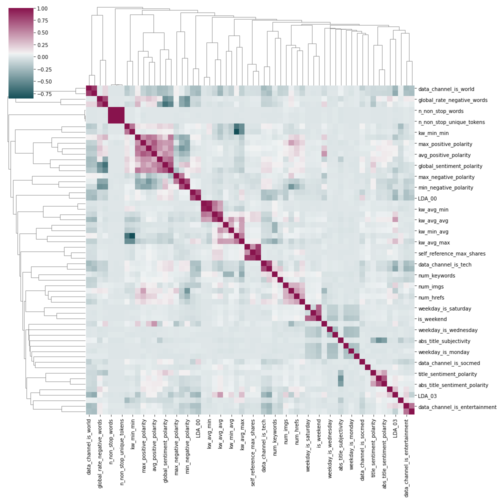
Corr-Pair-Plots and scales#
cmap = seaborn.diverging_palette(h_neg=210, h_pos=350, s=90, l=30, as_cmap=True, center="light")
seaborn.clustermap(data[numeric].corr(), figsize=(14, 14), cmap=cmap);
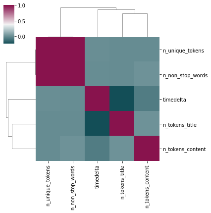
numeric[:5]
['timedelta',
 'n_tokens_title',
 'n_tokens_content',
 'n_unique_tokens',
 'n_non_stop_words']
data_numeric5 = data[numeric[:5]]
seaborn.clustermap(data_numeric5.corr(), figsize=(6, 6), cmap=cmap);
data_numeric5[::100].shape
(397, 5)
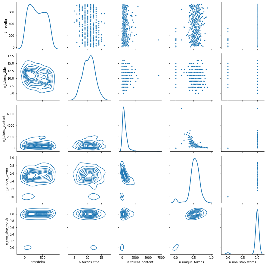
We take a subsample as the whole dataframe takes time to plot.
def my_pair_plot(df):
    g = seaborn.PairGrid(df, diag_sharey=False)
    g.map_upper(seaborn.scatterplot, s=15)
    g.map_lower(seaborn.kdeplot)
    g.map_diag(seaborn.kdeplot, lw=2)
    return g

my_pair_plot(data_numeric5[::100]);
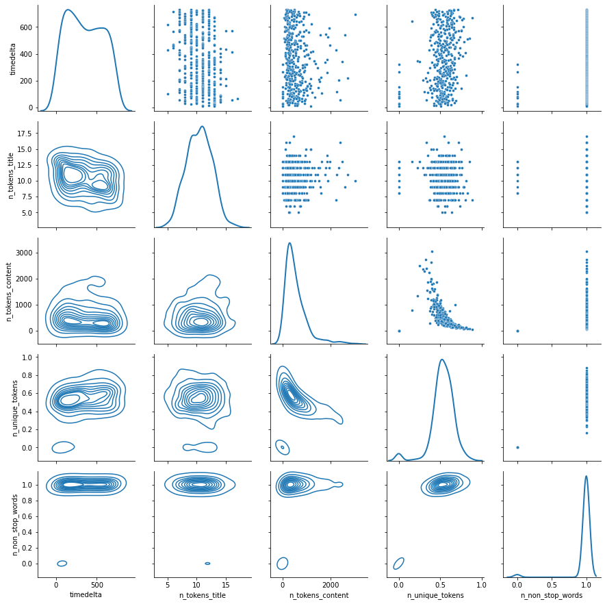
Or maybe it is because there are some outliers.
data[data.n_unique_tokens > 100]
| url | timedelta | n_tokens_title | n_tokens_content | n_unique_tokens | n_non_stop_words | n_non_stop_unique_tokens | num_hrefs | num_self_hrefs | num_imgs | ... | min_positive_polarity | max_positive_polarity | avg_negative_polarity | min_negative_polarity | max_negative_polarity | title_subjectivity | title_sentiment_polarity | abs_title_subjectivity | abs_title_sentiment_polarity | shares | |
|---|---|---|---|---|---|---|---|---|---|---|---|---|---|---|---|---|---|---|---|---|---|
| 31037 | http://mashable.com/2014/08/18/ukraine-civilia... | 142.0 | 9.0 | 1570.0 | 701.0 | 1042.0 | 650.0 | 11.0 | 10.0 | 51.0 | ... | 0.0 | 0.0 | 0.0 | 0.0 | 0.0 | 0.0 | 0.0 | 0.0 | 0.0 | 5900 |
1 rows × 61 columns
We remove this row as it seems an outliar:
data_clean = data[data.n_unique_tokens < 100].copy()
my_pair_plot(data_clean[numeric[:5]][::100]);
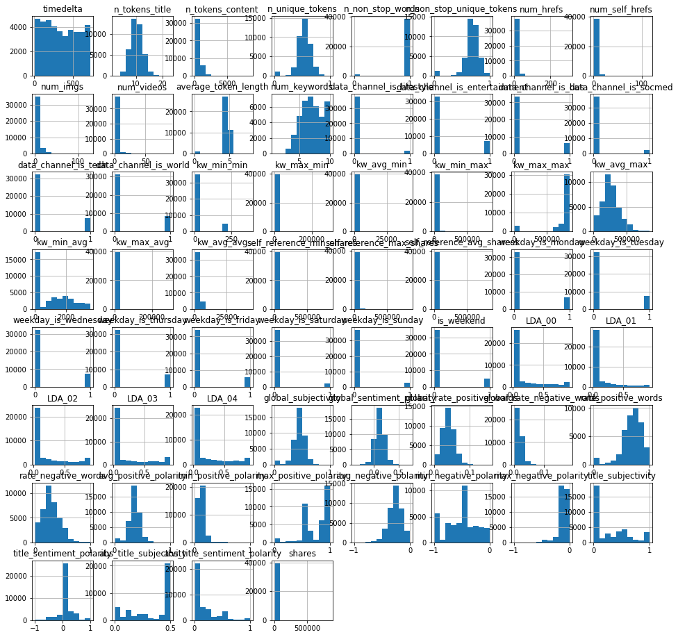
data_clean.hist(figsize=(16,16));
desc = data_clean.describe().T
desc["log"] = (desc["max"] > desc["50%"] * 9) & (desc["max"] > 1)
desc["scale"] = ""
desc.loc[desc["log"],"scale"] = "log"
desc[["mean", "min", "50%", "max", "scale"]]
| mean | min | 50% | max | scale | |
|---|---|---|---|---|---|
| timedelta | 354.535832 | 8.000000 | 339.000000 | 731.000000 | |
| n_tokens_title | 10.398784 | 2.000000 | 10.000000 | 23.000000 | |
| n_tokens_content | 546.488914 | 0.000000 | 409.000000 | 8474.000000 | log |
| n_unique_tokens | 0.530547 | 0.000000 | 0.539216 | 1.000000 | |
| n_non_stop_words | 0.970209 | 0.000000 | 1.000000 | 1.000000 | |
| n_non_stop_unique_tokens | 0.672796 | 0.000000 | 0.690476 | 1.000000 | |
| num_hrefs | 10.883687 | 0.000000 | 8.000000 | 304.000000 | log |
| num_self_hrefs | 3.293469 | 0.000000 | 3.000000 | 116.000000 | log |
| num_imgs | 4.542971 | 0.000000 | 1.000000 | 128.000000 | log |
| num_videos | 1.249905 | 0.000000 | 0.000000 | 91.000000 | log |
| average_token_length | 4.548236 | 0.000000 | 4.664078 | 8.041534 | |
| num_keywords | 7.223772 | 1.000000 | 7.000000 | 10.000000 | |
| data_channel_is_lifestyle | 0.052948 | 0.000000 | 0.000000 | 1.000000 | |
| data_channel_is_entertainment | 0.177989 | 0.000000 | 0.000000 | 1.000000 | |
| data_channel_is_bus | 0.157859 | 0.000000 | 0.000000 | 1.000000 | |
| data_channel_is_socmed | 0.058598 | 0.000000 | 0.000000 | 1.000000 | |
| data_channel_is_tech | 0.185304 | 0.000000 | 0.000000 | 1.000000 | |
| data_channel_is_world | 0.212572 | 0.000000 | 0.000000 | 1.000000 | |
| kw_min_min | 26.107484 | -1.000000 | -1.000000 | 377.000000 | log |
| kw_max_min | 1153.961166 | 0.000000 | 660.000000 | 298400.000000 | log |
| kw_avg_min | 312.371221 | -1.000000 | 235.500000 | 42827.857143 | log |
| kw_min_max | 13612.114774 | 0.000000 | 1400.000000 | 843300.000000 | log |
| kw_max_max | 752321.771813 | 0.000000 | 843300.000000 | 843300.000000 | |
| kw_avg_max | 259280.143039 | 0.000000 | 244566.666667 | 843300.000000 | |
| kw_min_avg | 1117.113731 | -1.000000 | 1023.619048 | 3613.039820 | |
| kw_max_avg | 5657.265804 | 0.000000 | 4355.694105 | 298400.000000 | log |
| kw_avg_avg | 3135.864283 | 0.000000 | 2870.047184 | 43567.659946 | log |
| self_reference_min_shares | 3998.836211 | 0.000000 | 1200.000000 | 843300.000000 | log |
| self_reference_max_shares | 10329.473218 | 0.000000 | 2800.000000 | 843300.000000 | log |
| self_reference_avg_sharess | 6401.684395 | 0.000000 | 2200.000000 | 843300.000000 | log |
| weekday_is_monday | 0.168025 | 0.000000 | 0.000000 | 1.000000 | |
| weekday_is_tuesday | 0.186389 | 0.000000 | 0.000000 | 1.000000 | |
| weekday_is_wednesday | 0.187549 | 0.000000 | 0.000000 | 1.000000 | |
| weekday_is_thursday | 0.183311 | 0.000000 | 0.000000 | 1.000000 | |
| weekday_is_friday | 0.143808 | 0.000000 | 0.000000 | 1.000000 | |
| weekday_is_saturday | 0.061877 | 0.000000 | 0.000000 | 1.000000 | |
| weekday_is_sunday | 0.069041 | 0.000000 | 0.000000 | 1.000000 | |
| is_weekend | 0.130918 | 0.000000 | 0.000000 | 1.000000 | |
| LDA_00 | 0.184604 | 0.018182 | 0.033387 | 0.926994 | |
| LDA_01 | 0.141259 | 0.018182 | 0.033345 | 0.925947 | |
| LDA_02 | 0.216326 | 0.018182 | 0.040004 | 0.919999 | |
| LDA_03 | 0.223775 | 0.018182 | 0.040001 | 0.926534 | |
| LDA_04 | 0.234035 | 0.018182 | 0.040727 | 0.927191 | |
| global_subjectivity | 0.443381 | 0.000000 | 0.453458 | 1.000000 | |
| global_sentiment_polarity | 0.119312 | -0.393750 | 0.119119 | 0.727841 | |
| global_rate_positive_words | 0.039626 | 0.000000 | 0.039024 | 0.155488 | |
| global_rate_negative_words | 0.016613 | 0.000000 | 0.015337 | 0.184932 | |
| rate_positive_words | 0.682167 | 0.000000 | 0.710526 | 1.000000 | |
| rate_negative_words | 0.287941 | 0.000000 | 0.280000 | 1.000000 | |
| avg_positive_polarity | 0.353834 | 0.000000 | 0.358760 | 1.000000 | |
| min_positive_polarity | 0.095448 | 0.000000 | 0.100000 | 1.000000 | |
| max_positive_polarity | 0.756747 | 0.000000 | 0.800000 | 1.000000 | |
| avg_negative_polarity | -0.259531 | -1.000000 | -0.253333 | 0.000000 | |
| min_negative_polarity | -0.521957 | -1.000000 | -0.500000 | 0.000000 | |
| max_negative_polarity | -0.107503 | -1.000000 | -0.100000 | 0.000000 | |
| title_subjectivity | 0.282360 | 0.000000 | 0.150000 | 1.000000 | |
| title_sentiment_polarity | 0.071427 | -1.000000 | 0.000000 | 1.000000 | |
| abs_title_subjectivity | 0.341851 | 0.000000 | 0.500000 | 0.500000 | |
| abs_title_sentiment_polarity | 0.156068 | 0.000000 | 0.000000 | 1.000000 | |
| shares | 3395.317004 | 1.000000 | 1400.000000 | 843300.000000 | log |
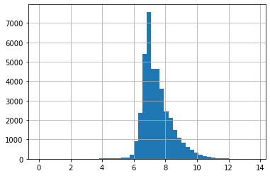
numpy.log(data_clean["shares"]).hist(bins=50);
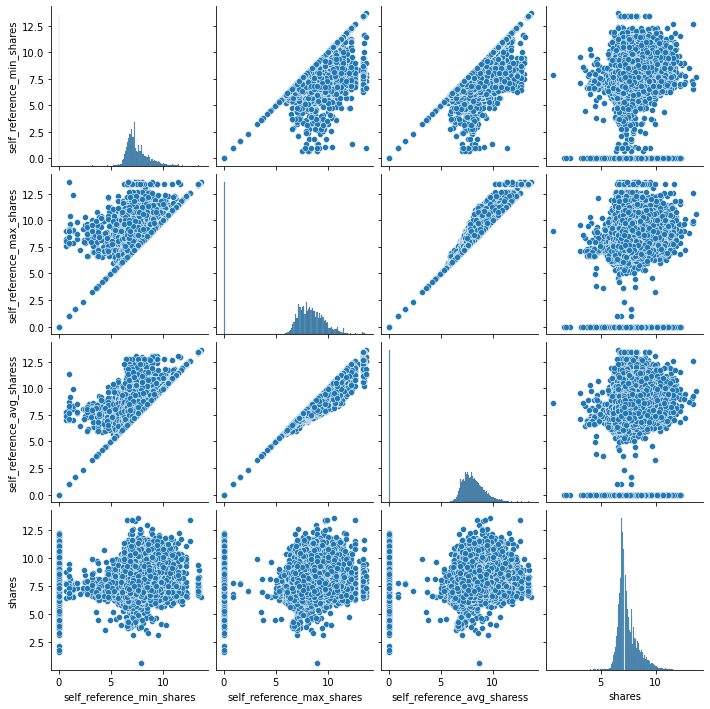
shares = data_clean[[c for c in numeric if "share" in c]].copy()
for c in shares.columns:
    shares[c] = numpy.log(shares[c] + 1)
seaborn.pairplot(shares);
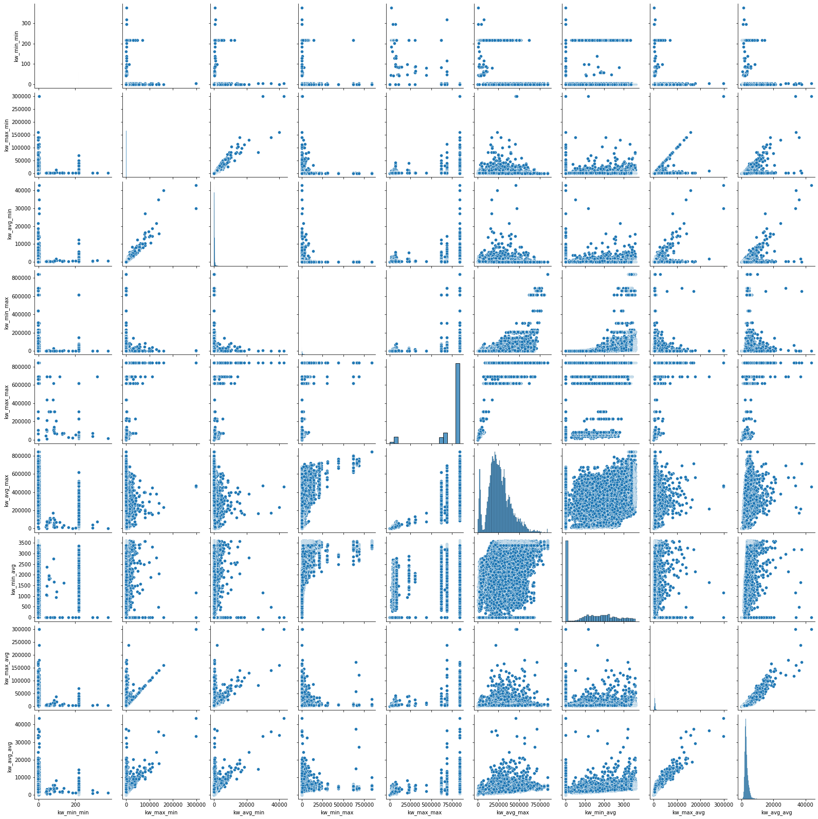
kw = data_clean[[c for c in numeric if "kw" in c]].copy()
seaborn.pairplot(kw);
Outcome, cleaning scaling#
cleaning
data_clean = data[data.n_unique_tokens < 100].copy()
scaling: we consider that if the maximum is far away from the mediane, the scale should be logarithmic as it is far way from a gaussian law, it just applies on this problem
desc = data_clean.describe().T
desc["log"] = (desc["max"] > desc["50%"] * 9) & (desc["max"] > 1)
desc["log+2"] = desc["log"] & (desc["min"] < 0)
desc["scale"] = ""
desc.loc[desc["log"],"scale"] = "log"
desc.loc[desc["log+2"],"scale"] = "log+2"
desc[["mean", "min", "50%", "max", "scale"]]
| mean | min | 50% | max | scale | |
|---|---|---|---|---|---|
| timedelta | 354.535832 | 8.000000 | 339.000000 | 731.000000 | |
| n_tokens_title | 10.398784 | 2.000000 | 10.000000 | 23.000000 | |
| n_tokens_content | 546.488914 | 0.000000 | 409.000000 | 8474.000000 | log |
| n_unique_tokens | 0.530547 | 0.000000 | 0.539216 | 1.000000 | |
| n_non_stop_words | 0.970209 | 0.000000 | 1.000000 | 1.000000 | |
| n_non_stop_unique_tokens | 0.672796 | 0.000000 | 0.690476 | 1.000000 | |
| num_hrefs | 10.883687 | 0.000000 | 8.000000 | 304.000000 | log |
| num_self_hrefs | 3.293469 | 0.000000 | 3.000000 | 116.000000 | log |
| num_imgs | 4.542971 | 0.000000 | 1.000000 | 128.000000 | log |
| num_videos | 1.249905 | 0.000000 | 0.000000 | 91.000000 | log |
| average_token_length | 4.548236 | 0.000000 | 4.664078 | 8.041534 | |
| num_keywords | 7.223772 | 1.000000 | 7.000000 | 10.000000 | |
| data_channel_is_lifestyle | 0.052948 | 0.000000 | 0.000000 | 1.000000 | |
| data_channel_is_entertainment | 0.177989 | 0.000000 | 0.000000 | 1.000000 | |
| data_channel_is_bus | 0.157859 | 0.000000 | 0.000000 | 1.000000 | |
| data_channel_is_socmed | 0.058598 | 0.000000 | 0.000000 | 1.000000 | |
| data_channel_is_tech | 0.185304 | 0.000000 | 0.000000 | 1.000000 | |
| data_channel_is_world | 0.212572 | 0.000000 | 0.000000 | 1.000000 | |
| kw_min_min | 26.107484 | -1.000000 | -1.000000 | 377.000000 | log+2 |
| kw_max_min | 1153.961166 | 0.000000 | 660.000000 | 298400.000000 | log |
| kw_avg_min | 312.371221 | -1.000000 | 235.500000 | 42827.857143 | log+2 |
| kw_min_max | 13612.114774 | 0.000000 | 1400.000000 | 843300.000000 | log |
| kw_max_max | 752321.771813 | 0.000000 | 843300.000000 | 843300.000000 | |
| kw_avg_max | 259280.143039 | 0.000000 | 244566.666667 | 843300.000000 | |
| kw_min_avg | 1117.113731 | -1.000000 | 1023.619048 | 3613.039820 | |
| kw_max_avg | 5657.265804 | 0.000000 | 4355.694105 | 298400.000000 | log |
| kw_avg_avg | 3135.864283 | 0.000000 | 2870.047184 | 43567.659946 | log |
| self_reference_min_shares | 3998.836211 | 0.000000 | 1200.000000 | 843300.000000 | log |
| self_reference_max_shares | 10329.473218 | 0.000000 | 2800.000000 | 843300.000000 | log |
| self_reference_avg_sharess | 6401.684395 | 0.000000 | 2200.000000 | 843300.000000 | log |
| weekday_is_monday | 0.168025 | 0.000000 | 0.000000 | 1.000000 | |
| weekday_is_tuesday | 0.186389 | 0.000000 | 0.000000 | 1.000000 | |
| weekday_is_wednesday | 0.187549 | 0.000000 | 0.000000 | 1.000000 | |
| weekday_is_thursday | 0.183311 | 0.000000 | 0.000000 | 1.000000 | |
| weekday_is_friday | 0.143808 | 0.000000 | 0.000000 | 1.000000 | |
| weekday_is_saturday | 0.061877 | 0.000000 | 0.000000 | 1.000000 | |
| weekday_is_sunday | 0.069041 | 0.000000 | 0.000000 | 1.000000 | |
| is_weekend | 0.130918 | 0.000000 | 0.000000 | 1.000000 | |
| LDA_00 | 0.184604 | 0.018182 | 0.033387 | 0.926994 | |
| LDA_01 | 0.141259 | 0.018182 | 0.033345 | 0.925947 | |
| LDA_02 | 0.216326 | 0.018182 | 0.040004 | 0.919999 | |
| LDA_03 | 0.223775 | 0.018182 | 0.040001 | 0.926534 | |
| LDA_04 | 0.234035 | 0.018182 | 0.040727 | 0.927191 | |
| global_subjectivity | 0.443381 | 0.000000 | 0.453458 | 1.000000 | |
| global_sentiment_polarity | 0.119312 | -0.393750 | 0.119119 | 0.727841 | |
| global_rate_positive_words | 0.039626 | 0.000000 | 0.039024 | 0.155488 | |
| global_rate_negative_words | 0.016613 | 0.000000 | 0.015337 | 0.184932 | |
| rate_positive_words | 0.682167 | 0.000000 | 0.710526 | 1.000000 | |
| rate_negative_words | 0.287941 | 0.000000 | 0.280000 | 1.000000 | |
| avg_positive_polarity | 0.353834 | 0.000000 | 0.358760 | 1.000000 | |
| min_positive_polarity | 0.095448 | 0.000000 | 0.100000 | 1.000000 | |
| max_positive_polarity | 0.756747 | 0.000000 | 0.800000 | 1.000000 | |
| avg_negative_polarity | -0.259531 | -1.000000 | -0.253333 | 0.000000 | |
| min_negative_polarity | -0.521957 | -1.000000 | -0.500000 | 0.000000 | |
| max_negative_polarity | -0.107503 | -1.000000 | -0.100000 | 0.000000 | |
| title_subjectivity | 0.282360 | 0.000000 | 0.150000 | 1.000000 | |
| title_sentiment_polarity | 0.071427 | -1.000000 | 0.000000 | 1.000000 | |
| abs_title_subjectivity | 0.341851 | 0.000000 | 0.500000 | 0.500000 | |
| abs_title_sentiment_polarity | 0.156068 | 0.000000 | 0.000000 | 1.000000 | |
| shares | 3395.317004 | 1.000000 | 1400.000000 | 843300.000000 | log |
import numpy
new_data = data_clean.copy()
for c in desc.index [ desc["scale"] == "log"]:
    new_data[c] = numpy.log(new_data[c] + 1)
for c in desc.index [ desc["scale"] == "log+2"]:
    new_data[c] = numpy.log(new_data[c] + 2)
new_data.shape
(39643, 61)
set(new_data.dtypes)
{dtype('float64'), dtype('O')}
from sklearn.model_selection import train_test_split

features = new_data[[c for c in numeric if c != "shares"]]
target = new_data["shares"]
X_train, X_test, y_train, y_test = train_test_split(features, target)
learning#
from sklearn.ensemble import RandomForestRegressor
clr = RandomForestRegressor(min_samples_leaf=20, n_estimators=50, min_weight_fraction_leaf=0.01, min_samples_split=10)
clr.fit(X_train, y_train)
RandomForestRegressor(min_samples_leaf=20, min_samples_split=10,
                      min_weight_fraction_leaf=0.01, n_estimators=50)
tpredicted = clr.predict(X_train)
df = pandas.DataFrame()
df["train_predicted"] = tpredicted
df["train_expected"] = y_train
df.corr()
| train_predicted | train_expected | |
|---|---|---|
| train_predicted | 1.000000 | 0.004091 |
| train_expected | 0.004091 | 1.000000 |
df = pandas.DataFrame()
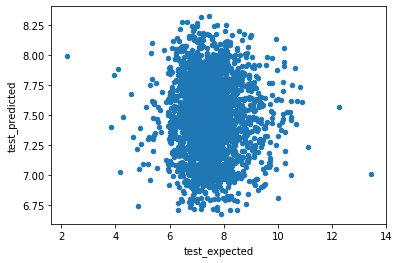
df["test_predicted"] = clr.predict(X_test)
df["test_expected"] = y_test
df.corr()
| test_predicted | test_expected | |
|---|---|---|
| test_predicted | 1.00000 | -0.00921 |
| test_expected | -0.00921 | 1.00000 |
df.plot(x ="test_expected", y="test_predicted", kind="scatter");
from sklearn.ensemble import GradientBoostingRegressor
est = GradientBoostingRegressor(min_samples_leaf=20, n_estimators=50, min_weight_fraction_leaf=0.01, min_samples_split=10)
est.fit(X_train, y_train)
GradientBoostingRegressor(min_samples_leaf=20, min_samples_split=10,
                          min_weight_fraction_leaf=0.01, n_estimators=50)
tpredicted = est.predict(X_train)
df = pandas.DataFrame()
df["train_predicted"] = tpredicted
df["train_expected"] = y_train
df.corr()
| train_predicted | train_expected | |
|---|---|---|
| train_predicted | 1.000000 | 0.008707 |
| train_expected | 0.008707 | 1.000000 |
df = pandas.DataFrame()
df["train_predicted"] = est.predict(X_train)
df["train_expected"] = y_train
df.corr()
| train_predicted | train_expected | |
|---|---|---|
| train_predicted | 1.000000 | 0.008707 |
| train_expected | 0.008707 | 1.000000 |
import xgboost
clxg = xgboost.XGBRegressor(max_depth=10, learning_rate=0.3, n_estimators=50)
clxg.fit(X_train, y_train)
XGBRegressor(base_score=0.5, booster='gbtree', colsample_bylevel=1,
             colsample_bynode=1, colsample_bytree=1, gamma=0, gpu_id=-1,
             importance_type='gain', interaction_constraints='',
             learning_rate=0.3, max_delta_step=0, max_depth=10,
             min_child_weight=1, missing=nan, monotone_constraints='()',
             n_estimators=50, n_jobs=0, num_parallel_tree=1, random_state=0,
             reg_alpha=0, reg_lambda=1, scale_pos_weight=1, subsample=1,
             tree_method='exact', validate_parameters=1, verbosity=None)
xgpredicted = clxg.predict(X_train)
df = pandas.DataFrame()
df["train_predicted"] = xgpredicted
df["train_expected"] = y_train
df.corr()
| train_predicted | train_expected | |
|---|---|---|
| train_predicted | 1.000000 | 0.000811 |
| train_expected | 0.000811 | 1.000000 |
# trop long
#from sklearn import tree
#from sklearn.ensemble import AdaBoostRegressor
#clfr = tree.DecisionTreeRegressor(min_samples_leaf=10, min_samples_split=10)
#clf2 = AdaBoostRegressor(clfr, n_estimators=800, learning_rate=0.5)
#clf2.fit(X_train, y_train)
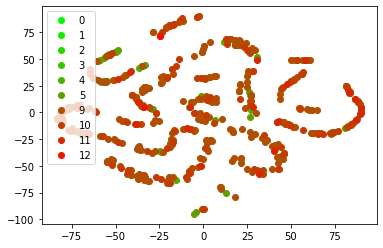
t-SNE#
Comparison of Manifold Learning methods, t-SNE, t-distributed Stochastic Neighbor Embedding (t-SNE)
from sklearn.model_selection import train_test_split
X_1, X_2, y_1, y_2 = train_test_split(X_train.reset_index(drop=True),
                        y_train.reset_index(drop=True), test_size=0.2, random_state=42)
X_1.shape, X_2.shape
((23785, 59), (5947, 59))
from sklearn.manifold import TSNE
model = TSNE(n_components=2, random_state=0)
model
TSNE(random_state=0)
W_2 = model.fit_transform(X_2)
i_2 = y_2.astype(int)
W_2.shape, X_2.shape, y_2.shape, i_2.shape
((5947, 2), (5947, 59), (5947,), (5947,))
mini, maxi = min(i_2), max(i_2)+1
import matplotlib.pyplot as plt
f, ax = plt.subplots()

for i in range(mini, maxi):
    ind = numpy.array(numpy.where(i_2==i)).T
    print(i, ind.shape)
    if i in(6,7,8):
        continue
    m = "o" if i <= 9 else "o"
    r = 1.0*i / maxi
    ax.plot(W_2[ind,0], W_2[ind,1], m, color =(r, 1-r, 0.0), label=str(i))
ax.legend()
ax;
0 (1, 1)
1 (1, 1)
2 (0, 1)
3 (3, 1)
4 (16, 1)
5 (38, 1)
6 (1821, 1)
7 (2646, 1)
8 (978, 1)
9 (321, 1)
10 (96, 1)
11 (24, 1)
12 (2, 1)