2A.ml - Séries temporelles - correction#
Links: notebook, html, python, slides, GitHub
Prédictions sur des séries temporelles.
from jyquickhelper import add_notebook_menu
add_notebook_menu()
%matplotlib inline
Une série temporelles#
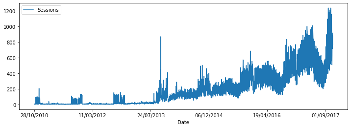
On récupère le nombre de sessions d’un site web.
import pandas
data = pandas.read_csv("xavierdupre_sessions.csv", sep="\t")
data.set_index("Date", inplace=True)
data.head()
| Sessions | |
|---|---|
| Date | |
| 28/10/2010 | 7 |
| 29/10/2010 | 6 |
| 30/10/2010 | 4 |
| 31/10/2010 | 6 |
| 01/11/2010 | 2 |
data.plot(figsize=(12,4));
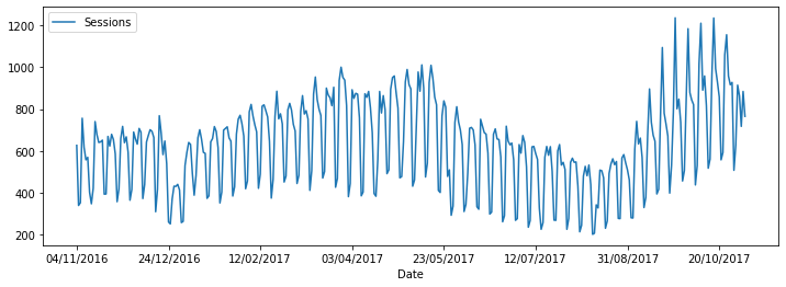
data[-365:].plot(figsize=(12,4));
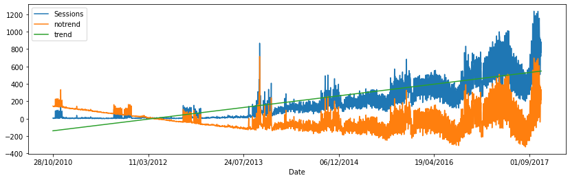
Trends#
Fonction detrend.
from statsmodels.tsa.tsatools import detrend
notrend = detrend(data['Sessions'])
data["notrend"] = notrend
data["trend"] = data['Sessions'] - notrend
data.tail()
| Sessions | notrend | trend | |
|---|---|---|---|
| Date | |||
| 30/10/2017 | 914 | 367.387637 | 546.612363 |
| 31/10/2017 | 863 | 316.119822 | 546.880178 |
| 01/11/2017 | 717 | 169.852008 | 547.147992 |
| 02/11/2017 | 884 | 336.584193 | 547.415807 |
| 03/11/2017 | 765 | 217.316379 | 547.683621 |
data.plot(y=["Sessions", "notrend", "trend"], figsize=(14,4));
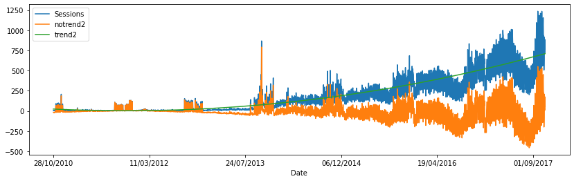
On essaye de calculer une tendance en minimisant :
 .
.
notrend2 = detrend(data['Sessions'], order=2)
data["notrend2"] = notrend2
data["trend2"] = data["Sessions"] - data["notrend2"]
data.plot(y=["Sessions", "notrend2", "trend2"], figsize=(14,4));
On passe au log.
import numpy
data["logSess"] = data["Sessions"].apply(lambda x: numpy.log(x+1))
lognotrend = detrend(data['logSess'])
data["lognotrend"] = lognotrend
data["logtrend"] = data["logSess"] - data["lognotrend"]
data.plot(y=["logSess", "lognotrend", "logtrend"], figsize=(14,4));
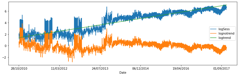
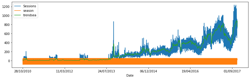
La série est assez particulière. Elle donne l’impression d’avoir un changement de régime. On extrait la composante saisonnière avec seasonal_decompose.
from statsmodels.tsa.seasonal import seasonal_decompose
res = seasonal_decompose(data["Sessions"].values.ravel(), freq=7, two_sided=False)
data["season"] = res.seasonal
data["trendsea"] = res.trend
data.plot(y=["Sessions", "season", "trendsea"], figsize=(14,4));
<ipython-input-23-986850a44b5e>:2: FutureWarning: the 'freq'' keyword is deprecated, use 'period' instead.
  res = seasonal_decompose(data["Sessions"].values.ravel(), freq=7, two_sided=False)
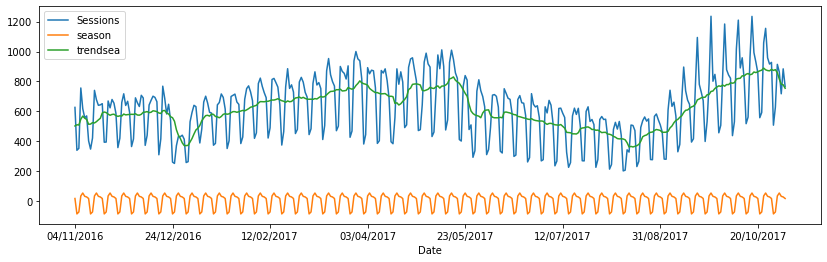
data[-365:].plot(y=["Sessions", "season", "trendsea"], figsize=(14,4));
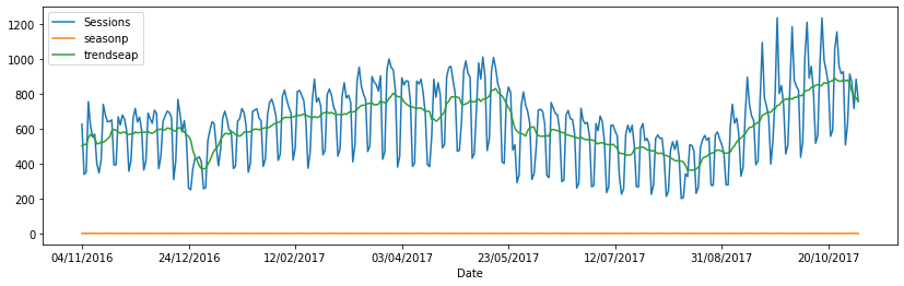
res = seasonal_decompose(data["Sessions"].values.ravel() + 1, freq=7,
                         two_sided=False, model='multiplicative')
data["seasonp"] = res.seasonal
data["trendseap"] = res.trend
data[-365:].plot(y=["Sessions", "seasonp", "trendseap"], figsize=(14,4));
<ipython-input-25-c64a8f19748f>:1: FutureWarning: the 'freq'' keyword is deprecated, use 'period' instead.
  res = seasonal_decompose(data["Sessions"].values.ravel() + 1, freq=7,
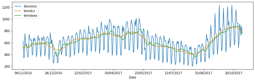
Enlever la saisonnalité sans la connaître#
Avec fit_seasons.
from seasonal import fit_seasons
cv_seasons, trend = fit_seasons(data["Sessions"])
print(cv_seasons)
# data["cs_seasons"] = cv_seasons
data["trendcs"] = trend
data[-365:].plot(y=["Sessions", "trendcs", "trendsea"], figsize=(14,4));
[ 26.66213008  16.33420353 -86.59519495 -73.57497492  33.23110565
  52.87820674  30.87516435]
Autocorrélograme#
On s’inspire de l’exemple : Autoregressive Moving Average (ARMA): Sunspots data.
import matplotlib.pyplot as plt
from statsmodels.graphics.tsaplots import plot_acf, plot_pacf
fig = plt.figure(figsize=(12,8))
ax1 = fig.add_subplot(211)
fig = plot_acf(data["Sessions"], lags=40, ax=ax1)
ax2 = fig.add_subplot(212)
fig = plot_pacf(data["Sessions"], lags=40, ax=ax2);
C:Python395_x64libsite-packagesstatsmodelstsabasetsa_model.py:7: FutureWarning: pandas.Int64Index is deprecated and will be removed from pandas in a future version. Use pandas.Index with the appropriate dtype instead.
  from pandas import (to_datetime, Int64Index, DatetimeIndex, Period,
C:Python395_x64libsite-packagesstatsmodelstsabasetsa_model.py:7: FutureWarning: pandas.Float64Index is deprecated and will be removed from pandas in a future version. Use pandas.Index with the appropriate dtype instead.
  from pandas import (to_datetime, Int64Index, DatetimeIndex, Period,
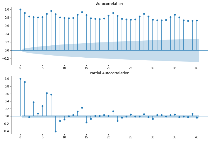
On retrouve bien une période de 7.