Train a linear regression with onnxruntime-training

This example explores how onnxruntime-training can be used to train a simple linear regression using a gradient descent. It compares the results with those obtained by sklearn.linear_model.LinearRegression.

A simple linear regression with scikit-learn

from pprint import pprint
import numpy as np
from pandas import DataFrame
from onnx import helper, numpy_helper, TensorProto
from onnx.tools.net_drawer import GetPydotGraph, GetOpNodeProducer
from onnxruntime import (
    InferenceSession, __version__ as ort_version,
    TrainingParameters, SessionOptions, TrainingSession)
import matplotlib.pyplot as plt
from pyquickhelper.helpgen.graphviz_helper import plot_graphviz
from sklearn.datasets import make_regression
from sklearn.model_selection import train_test_split
from sklearn.linear_model import LinearRegression
from tqdm import tqdm

X, y = make_regression(n_features=2, bias=2)
X = X.astype(np.float32)
y = y.astype(np.float32)
X_train, X_test, y_train, y_test = train_test_split(X, y)

lr = LinearRegression()
lr.fit(X, y)
print(lr.predict(X[:5]))

[-34.349747  -81.39873    -1.1478987  -4.6620636  11.685635 ]

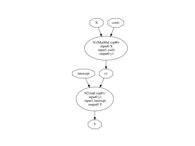
An equivalent ONNX graph.

This graph can be obtained with *sklearn-onnx` as we need to modify it for training, it is easier to create an explicit one.

def onnx_linear_regression(coefs, intercept):
    if len(coefs.shape) == 1:
        coefs = coefs.reshape((1, -1))
    coefs = coefs.T

    # input and output
    X = helper.make_tensor_value_info(
        'X', TensorProto.FLOAT, [None, coefs.shape[0]])
    Y = helper.make_tensor_value_info(
        'Y', TensorProto.FLOAT, [None, coefs.shape[1]])

    # inference
    node_matmul = helper.make_node('MatMul', ['X', 'coefs'], ['y1'], name='N1')
    node_add = helper.make_node('Add', ['y1', 'intercept'], ['Y'], name='N2')

    # initializer
    init_coefs = numpy_helper.from_array(coefs, name="coefs")
    init_intercept = numpy_helper.from_array(intercept, name="intercept")

    # graph
    graph_def = helper.make_graph(
        [node_matmul, node_add], 'lr', [X], [Y],
        [init_coefs, init_intercept])
    model_def = helper.make_model(
        graph_def, producer_name='orttrainer', ir_version=7,
        producer_version=ort_version,
        opset_imports=[helper.make_operatorsetid('', 14)])
    return model_def


onx = onnx_linear_regression(lr.coef_.astype(np.float32),
                             lr.intercept_.astype(np.float32))

Let’s visualize it.

def plot_dot(model):
    pydot_graph = GetPydotGraph(
        model.graph, name=model.graph.name, rankdir="TB",
        node_producer=GetOpNodeProducer("docstring"))
    return plot_graphviz(pydot_graph.to_string())

plot_dot(onx)

<AxesSubplot: >

We check it produces the same outputs.

sess = InferenceSession(onx.SerializeToString())
print(sess.run(None, {'X': X[:5]})[0])

[[-34.349747 ]
 [-81.39873  ]
 [ -1.1478987]
 [ -4.6620636]
 [ 11.685635 ]]

It works.

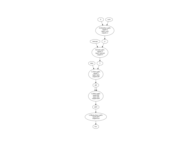
Training with onnxruntime-training

It is possible only if the graph to train has a gradient. Then the model can be trained with a gradient descent algorithm. The previous graph only predicts, a new graph needs to be created to compute the loss as well. In our case, it is a square loss. The new graph requires another input for the label and another output for the loss value.

def onnx_linear_regression_training(coefs, intercept):
    if len(coefs.shape) == 1:
        coefs = coefs.reshape((1, -1))
    coefs = coefs.T

    # input
    X = helper.make_tensor_value_info(
        'X', TensorProto.FLOAT, [None, coefs.shape[0]])

    # expected input
    label = helper.make_tensor_value_info(
        'label', TensorProto.FLOAT, [None, coefs.shape[1]])

    # output
    Y = helper.make_tensor_value_info(
        'Y', TensorProto.FLOAT, [None, coefs.shape[1]])

    # loss
    loss = helper.make_tensor_value_info('loss', TensorProto.FLOAT, [])

    # inference
    node_matmul = helper.make_node('MatMul', ['X', 'coefs'], ['y1'], name='N1')
    node_add = helper.make_node('Add', ['y1', 'intercept'], ['Y'], name='N2')

    # loss
    node_diff = helper.make_node('Sub', ['Y', 'label'], ['diff'], name='L1')
    node_square = helper.make_node(
        'Mul', ['diff', 'diff'], ['diff2'], name='L2')
    node_square_sum = helper.make_node(
        'ReduceSum', ['diff2'], ['loss'], name='L3')

    # initializer
    init_coefs = numpy_helper.from_array(coefs, name="coefs")
    init_intercept = numpy_helper.from_array(intercept, name="intercept")

    # graph
    graph_def = helper.make_graph(
        [node_matmul, node_add, node_diff, node_square, node_square_sum],
        'lrt', [X, label], [loss, Y], [init_coefs, init_intercept])
    model_def = helper.make_model(
        graph_def, producer_name='orttrainer', ir_version=7,
        producer_version=ort_version,
        opset_imports=[helper.make_operatorsetid('', 14)])
    return model_def

We create a graph with random coefficients.

onx_train = onnx_linear_regression_training(
    np.random.randn(*lr.coef_.shape).astype(np.float32),
    np.random.randn(*lr.intercept_.reshape((-1, )).shape).astype(np.float32))

plot_dot(onx_train)

<AxesSubplot: >

DataLoader

Next class draws consecutive random observations from a dataset by batch.

class DataLoader:
    """
    Draws consecutive random observations from a dataset
    by batch. It iterates over the datasets by drawing
    *batch_size* consecutive observations.

    :param X: features
    :param y: labels
    :param batch_size: batch size (consecutive observations)
    """

    def __init__(self, X, y, batch_size=20):
        self.X, self.y = X, y
        self.batch_size = batch_size
        if len(self.y.shape) == 1:
            self.y = self.y.reshape((-1, 1))
        if self.X.shape[0] != self.y.shape[0]:
            raise ValueError(
                "Shape mismatch X.shape=%r, y.shape=%r." % (
                    self.X.shape, self.y.shape))

    def __len__(self):
        "Returns the number of observations."
        return self.X.shape[0]

    def __iter__(self):
        """
        Iterates over the datasets by drawing
        *batch_size* consecutive observations.
        """
        N = 0
        b = len(self) - self.batch_size
        while N < len(self):
            i = np.random.randint(0, b)
            N += self.batch_size
            yield (self.X[i:i + self.batch_size],
                   self.y[i:i + self.batch_size])

    @property
    def data(self):
        "Returns a tuple of the datasets."
        return self.X, self.y


data_loader = DataLoader(X_train, y_train, batch_size=2)


for i, batch in enumerate(data_loader):
    if i >= 2:
        break
    print("batch %r: %r" % (i, batch))

batch 0: (array([[ 0.06440964,  0.18517685],
       [-1.7677377 , -0.59794754]], dtype=float32), array([[ 11.284166],
       [-96.02698 ]], dtype=float32))
batch 1: (array([[-2.2048771 ,  1.6949888 ],
       [ 0.20187879,  0.90629065]], dtype=float32), array([[-34.93256 ],
       [ 42.493137]], dtype=float32))

First iterations of training

Prediction needs an instance of class InferenceSession, the training needs an instance of class TrainingSession. Next function creates this one.

def create_training_session(
        training_onnx, weights_to_train, loss_output_name='loss',
        training_optimizer_name='SGDOptimizer'):
    """
    Creates an instance of class `TrainingSession`.

    :param training_onnx: ONNX graph used to train
    :param weights_to_train: names of initializers to be optimized
    :param loss_output_name: name of the loss output
    :param training_optimizer_name: optimizer name
    :return: instance of `TrainingSession`
    """
    ort_parameters = TrainingParameters()
    ort_parameters.loss_output_name = loss_output_name
    ort_parameters.use_mixed_precision = False


    output_types = {}
    for output in training_onnx.graph.output:
        output_types[output.name] = output.type.tensor_type

    ort_parameters.weights_to_train = set(weights_to_train)
    ort_parameters.training_optimizer_name = training_optimizer_name
    # ort_parameters.lr_params_feed_name = lr_params_feed_name

    ort_parameters.optimizer_attributes_map = {
        name: {} for name in weights_to_train}
    ort_parameters.optimizer_int_attributes_map = {
        name: {} for name in weights_to_train}

    session_options = SessionOptions()
    session_options.use_deterministic_compute = True

    session = TrainingSession(
        training_onnx.SerializeToString(), ort_parameters, session_options)
    return session


train_session = create_training_session(onx_train, ['coefs', 'intercept'])
print(train_session)

<onnxruntime.capi.training.training_session.TrainingSession object at 0x7f0302fdfd60>

Let’s look into the expected inputs and outputs.

for i in train_session.get_inputs():
    print("+input: %s (%s%s)" % (i.name, i.type, i.shape))
for o in train_session.get_outputs():
    print("output: %s (%s%s)" % (o.name, o.type, o.shape))

+input: X (tensor(float)[None, 2])
+input: label (tensor(float)[None, 1])
+input: Learning_Rate (tensor(float)[1])
output: loss (tensor(float)[1, 1])
output: Y (tensor(float)[None, 1])
output: global_gradient_norm (tensor(float)[])

A third parameter Learning_Rate was added. The training updates the weight with a gradient multiplied by this parameter. Let’s see now how to retrieve the trained coefficients.

state_tensors = train_session.get_state()
pprint(state_tensors)

{'coefs': array([[-0.07605116],
       [ 0.35835147]], dtype=float32),
 'intercept': array([-0.5061662], dtype=float32)}

We can now check the coefficients are updated after one iteration.

inputs = {'X': X_train[:1],
          'label': y_train[:1].reshape((-1, 1)),
          'Learning_Rate': np.array([0.001], dtype=np.float32)}

train_session.run(None, inputs)
state_tensors = train_session.get_state()
pprint(state_tensors)

{'coefs': array([[-0.03618829],
       [ 0.38130143]], dtype=float32),
 'intercept': array([-0.5749262], dtype=float32)}

They changed. Another iteration to be sure.

inputs = {'X': X_train[:1],
          'label': y_train[:1].reshape((-1, 1)),
          'Learning_Rate': np.array([0.001], dtype=np.float32)}
res = train_session.run(None, inputs)
state_tensors = train_session.get_state()
pprint(state_tensors)

{'coefs': array([[0.00355918],
       [0.40418497]], dtype=float32),
 'intercept': array([-0.6434871], dtype=float32)}

It works. The training loss can be obtained by looking into the results.

pprint(res)

[array([[1175.1499]], dtype=float32),
 array([[-0.68121314]], dtype=float32),
 array(82.48707, dtype=float32)]

Training

We need to implement a gradient descent. Let’s wrap this into a class similar following scikit-learn’s API.

class CustomTraining:
    """
    Implements a simple :epkg:`Stochastic Gradient Descent`.

    :param model_onnx: ONNX graph to train
    :param weights_to_train: list of initializers to train
    :param loss_output_name: name of output loss
    :param max_iter: number of training iterations
    :param training_optimizer_name: optimizing algorithm
    :param batch_size: batch size (see class *DataLoader*)
    :param eta0: initial learning rate for the `'constant'`, `'invscaling'`
        or `'adaptive'` schedules.
    :param alpha: constant that multiplies the regularization term,
        the higher the value, the stronger the regularization.
        Also used to compute the learning rate when set to *learning_rate*
        is set to `'optimal'`.
    :param power_t: exponent for inverse scaling learning rate
    :param learning_rate: learning rate schedule:
        * `'constant'`: `eta = eta0`
        * `'optimal'`: `eta = 1.0 / (alpha * (t + t0))` where *t0* is chosen
            by a heuristic proposed by Leon Bottou.
        * `'invscaling'`: `eta = eta0 / pow(t, power_t)`
    :param verbose: use :epkg:`tqdm` to display the training progress
    """
    def __init__(self, model_onnx, weights_to_train, loss_output_name='loss',
                 max_iter=100, training_optimizer_name='SGDOptimizer', batch_size=10,
                 eta0=0.01, alpha=0.0001, power_t=0.25, learning_rate='invscaling',
                 verbose=0):
        # See https://scikit-learn.org/stable/modules/generated/
        # sklearn.linear_model.SGDRegressor.html
        self.model_onnx = model_onnx
        self.batch_size = batch_size
        self.weights_to_train = weights_to_train
        self.loss_output_name = loss_output_name
        self.training_optimizer_name = training_optimizer_name
        self.verbose = verbose
        self.max_iter = max_iter
        self.eta0 = eta0
        self.alpha = alpha
        self.power_t = power_t
        self.learning_rate = learning_rate.lower()

    def _init_learning_rate(self):
        self.eta0_ = self.eta0
        if self.learning_rate == "optimal":
            typw = np.sqrt(1.0 / np.sqrt(self.alpha))
            self.eta0_ = typw / max(1.0, (1 + typw) * 2)
            self.optimal_init_ = 1.0 / (self.eta0_ * self.alpha)
        else:
            self.eta0_ = self.eta0
        return self.eta0_

    def _update_learning_rate(self, t, eta):
        if self.learning_rate == "optimal":
            eta = 1.0 / (self.alpha * (self.optimal_init_ + t))
        elif self.learning_rate == "invscaling":
            eta = self.eta0_ / np.power(t + 1, self.power_t)
        return eta

    def fit(self, X, y):
        """
        Trains the model.
        :param X: features
        :param y: expected output
        :return: self
        """
        self.train_session_ = create_training_session(
            self.model_onnx, self.weights_to_train,
            loss_output_name=self.loss_output_name,
            training_optimizer_name=self.training_optimizer_name)

        data_loader = DataLoader(X, y, batch_size=self.batch_size)
        lr = self._init_learning_rate()
        self.input_names_ = [i.name for i in self.train_session_.get_inputs()]
        self.output_names_ = [
            o.name for o in self.train_session_.get_outputs()]
        self.loss_index_ = self.output_names_.index(self.loss_output_name)

        loop = (
            tqdm(range(self.max_iter))
            if self.verbose else range(self.max_iter))
        train_losses = []
        for it in loop:
            loss = self._iteration(data_loader, lr)
            lr = self._update_learning_rate(it, lr)
            if self.verbose > 1:
                loop.set_description("loss=%1.3g lr=%1.3g" % (loss, lr))
            train_losses.append(loss)
        self.train_losses_ = train_losses
        self.trained_coef_ = self.train_session_.get_state()
        return self

    def _iteration(self, data_loader, learning_rate):
        """
        Processes one gradient iteration.

        :param data_lower: instance of class `DataLoader`
        :return: loss
        """
        actual_losses = []
        lr = np.array([learning_rate], dtype=np.float32)
        for batch_idx, (data, target) in enumerate(data_loader):
            if len(target.shape) == 1:
                target = target.reshape((-1, 1))

            inputs = {self.input_names_[0]: data,
                      self.input_names_[1]: target,
                      self.input_names_[2]: lr}
            res = self.train_session_.run(None, inputs)
            actual_losses.append(res[self.loss_index_])
        return np.array(actual_losses).mean()

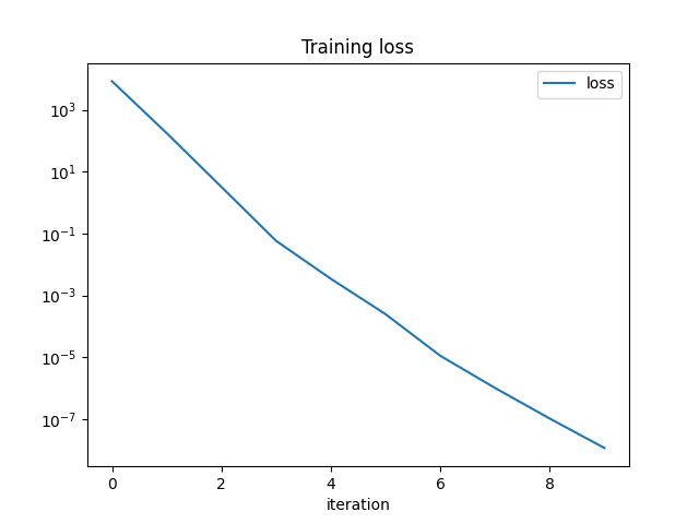
Let’s now train the model in a very similar way that it would be done with scikit-learn.

trainer = CustomTraining(onx_train, ['coefs', 'intercept'], verbose=1,
                         max_iter=10)
trainer.fit(X, y)
print("training losses:", trainer.train_losses_)

df = DataFrame({"iteration": np.arange(len(trainer.train_losses_)),
                "loss": trainer.train_losses_})
df.set_index('iteration').plot(title="Training loss", logy=True)

  0%|          | 0/10 [00:00<?, ?it/s]
100%|##########| 10/10 [00:00<00:00, 340.39it/s]
training losses: [8459.656, 176.5693, 3.2292314, 0.05809601, 0.0034594808, 0.00024783175, 1.1203884e-05, 1.0228407e-06, 1.046408e-07, 1.1679669e-08]

<AxesSubplot: title={'center': 'Training loss'}, xlabel='iteration'>

Let’s compare scikit-learn trained coefficients and the coefficients obtained with onnxruntime and check they are very close.

print("scikit-learn", lr.coef_, lr.intercept_)
print("onnxruntime", trainer.trained_coef_)

scikit-learn [43.62726  34.961987] 2.000001
onnxruntime {'coefs': array([[43.627243],
       [34.96198 ]], dtype=float32), 'intercept': array([2.0000107], dtype=float32)}

It works. We could stop here or we could update the weights in the training model or the first model. That requires to update the constants in an ONNX graph. We could also compares the algorithm processing time to scikit-learn or pytorch.

Update weights in an ONNX graph

Let’s first check the output of the first model in ONNX.

sess = InferenceSession(onx.SerializeToString())
before = sess.run(None, {'X': X[:5]})[0]
print(before)

[[-34.349747 ]
 [-81.39873  ]
 [ -1.1478987]
 [ -4.6620636]
 [ 11.685635 ]]

Let’s replace the initializer.

def update_onnx_graph(model_onnx, new_weights):
    replace_weights = []
    replace_indices = []
    for i, w in enumerate(model_onnx.graph.initializer):
        if w.name in new_weights:
            replace_weights.append(
                numpy_helper.from_array(new_weights[w.name], w.name))
            replace_indices.append(i)
    replace_indices.sort(reverse=True)
    for w_i in replace_indices:
        del model_onnx.graph.initializer[w_i]
    model_onnx.graph.initializer.extend(replace_weights)


update_onnx_graph(onx, trainer.trained_coef_)

Let’s compare with the previous output.

sess = InferenceSession(onx.SerializeToString())
after = sess.run(None, {'X': X[:5]})[0]
print(after)

[[-34.34972  ]
 [-81.39869  ]
 [ -1.1478851]
 [ -4.662055 ]
 [ 11.68564  ]]

It looks almost the same but slighly different.

print(after - before)

[[2.6702881e-05]
 [3.8146973e-05]
 [1.3589859e-05]
 [8.5830688e-06]
 [5.7220459e-06]]

Next example will show how to train a linear regression on GPU: Train a linear regression with onnxruntime-training on GPU.