Deploy machine learned models with ONNX#
Links: notebook, html, PDF, python, slides, GitHub
Xavier Dupré - Senior Data Scientist at Microsoft - Computer Science Teacher at ENSAE
Most of machine learning libraries are optimized to train models and not necessarily to use them for fast predictions in online web services. ONNX is one solution started last year by Microsoft and Facebook. This presentation describes the concept and shows some examples with scikit-learn and ML.net.
GitHub repos
Contributing to
from jyquickhelper import add_notebook_menu
add_notebook_menu(last_level=2)
%matplotlib inline
import matplotlib.pyplot as plt
from pyquickhelper.helpgen import NbImage
Open source tools in this talk#
import keras, lightgbm, onnx, skl2onnx, onnxruntime, sklearn, torch, xgboost
mods = [keras, lightgbm, onnx, skl2onnx, onnxruntime, sklearn, torch, xgboost]
for m in mods:
    print(m.__name__, m.__version__)
Using TensorFlow backend.
keras 2.3.1
lightgbm 2.3.1
onnx 1.7.105
skl2onnx 1.7.0
onnxruntime 1.3.993
sklearn 0.24.dev0
torch 1.5.0+cpu
xgboost 1.1.0
The problem about deployment#
Learn and predict#
Two different purposes not necessarily aligned for optimization
Learn : computation optimized for large number of observations (batch prediction)
Predict : computation optimized for one observation (one-off prediction)
Machine learning libraries optimize the learn scenario.
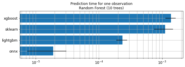
One-off prediction with random forests#
Benchmark of libraries for a regression problem.
from sklearn.datasets import load_diabetes
diabetes = load_diabetes()
diabetes_X_train = diabetes.data[:-20]
diabetes_X_test  = diabetes.data[-20:]
diabetes_y_train = diabetes.target[:-20]
diabetes_y_test  = diabetes.target[-20:]
diabetes_X_train[:1]
array([[ 0.03807591,  0.05068012,  0.06169621,  0.02187235, -0.0442235 ,
        -0.03482076, -0.04340085, -0.00259226,  0.01990842, -0.01764613]])
from jupytalk.benchmark import make_dataframe
df = make_dataframe(diabetes_y_train, diabetes_X_train)
df.to_csv("diabetes.csv", index=False)
df.head(n=2)
| Label | F0 | F1 | F2 | F3 | F4 | F5 | F6 | F7 | F8 | F9 | |
|---|---|---|---|---|---|---|---|---|---|---|---|
| 0 | 151.0 | 0.038076 | 0.050680 | 0.061696 | 0.021872 | -0.044223 | -0.034821 | -0.043401 | -0.002592 | 0.019908 | -0.017646 |
| 1 | 75.0 | -0.001882 | -0.044642 | -0.051474 | -0.026328 | -0.008449 | -0.019163 | 0.074412 | -0.039493 | -0.068330 | -0.092204 |
from jupytalk.benchmark import timeexec
measures_rf = []
from sklearn.ensemble import RandomForestRegressor
rf = RandomForestRegressor(n_estimators=10)
rf.fit(diabetes_X_train, diabetes_y_train)
RandomForestRegressor(n_estimators=10)
measures_rf += [timeexec("sklearn", "rf.predict(diabetes_X_test[:1])",
                         context=globals())]
Average: 1.11 ms deviation 369.54 µs (with 50 runs) in [846.82 µs, 1.98 ms]
from xgboost import XGBRegressor
xg = XGBRegressor(n_estimators=10)
xg.fit(diabetes_X_train, diabetes_y_train)
XGBRegressor(base_score=0.5, booster='gbtree', colsample_bylevel=1,
             colsample_bynode=1, colsample_bytree=1, gamma=0, gpu_id=-1,
             importance_type='gain', interaction_constraints='',
             learning_rate=0.300000012, max_delta_step=0, max_depth=6,
             min_child_weight=1, missing=nan, monotone_constraints='()',
             n_estimators=10, n_jobs=0, num_parallel_tree=1, random_state=0,
             reg_alpha=0, reg_lambda=1, scale_pos_weight=1, subsample=1,
             tree_method='exact', validate_parameters=1, verbosity=None)
measures_rf += [timeexec("xgboost", "xg.predict(diabetes_X_test[:1])",
                         context=globals())]
Average: 1.38 ms deviation 251.41 µs (with 50 runs) in [1.18 ms, 1.98 ms]
from lightgbm import LGBMRegressor
lg = LGBMRegressor(n_estimators=10)
lg.fit(diabetes_X_train, diabetes_y_train)
LGBMRegressor(n_estimators=10)
measures_rf += [timeexec("lightgbm", "lg.predict(diabetes_X_test[:1])",
                         context=globals())]
Average: 234.68 µs deviation 45.85 µs (with 50 runs) in [193.29 µs, 313.33 µs]
This would require to reimplement the prediction function.
import pandas
df = pandas.DataFrame(data=measures_rf)
df = df.set_index("legend").sort_values("average")
df
| average | deviation | first | first3 | last3 | repeat | min5 | max5 | code | run | |
|---|---|---|---|---|---|---|---|---|---|---|
| legend | ||||||||||
| lightgbm | 0.000235 | 0.000046 | 0.000499 | 0.000348 | 0.000257 | 200 | 0.000193 | 0.000313 | lg.predict(diabetes_X_test[:1]) | 50 |
| sklearn | 0.001113 | 0.000370 | 0.001451 | 0.001219 | 0.000916 | 200 | 0.000847 | 0.001982 | rf.predict(diabetes_X_test[:1]) | 50 |
| xgboost | 0.001377 | 0.000251 | 0.002161 | 0.001656 | 0.001348 | 200 | 0.001183 | 0.001982 | xg.predict(diabetes_X_test[:1]) | 50 |
%matplotlib inline
import matplotlib.pyplot as plt
fig, ax = plt.subplots(1, 1, figsize=(10,3))
df[["average", "deviation"]].plot(kind="barh", logx=True, ax=ax, xerr="deviation",
                                  legend=False, fontsize=12, width=0.8)
ax.set_ylabel("")
ax.grid(b=True, which="major")
ax.grid(b=True, which="minor")
ax.set_title("Prediction time for one observation\nRandom Forest (10 trees)");
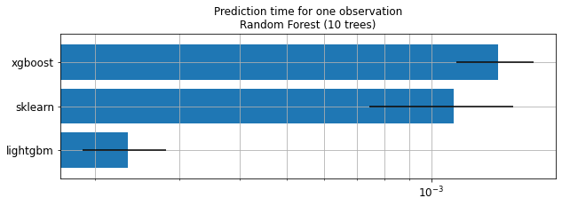
Keep in mind
Trained trees are not necessarily the same.
Performance is not compared.
Order of magnitude is important here.
What is batch prediction?#
Instead of running
 times 1 prediction
We run 1 time
predictions
The code can be found at MS Experience 2018.
NbImage('batch.png', width=600)

ONNX#
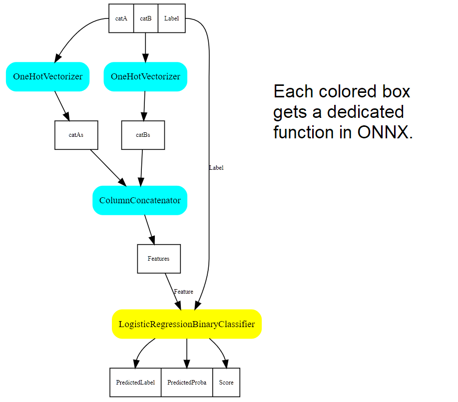
ONNX can represent any pipeline of data.
Let’s visualize a machine learning pipeline (see the code at MS Experience).
NbImage("pipeviz.png", width=500)
ONNX = language to describe models#
Standard format to describe machine learning
Easier to exchange, export
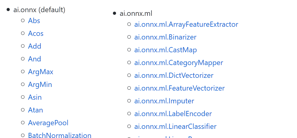
ONNX = machine learning oriented#
Can represent any mathematical function handling numerical and text features.
NbImage("onnxop.png", width=600)
ONNX = efficient serialization#
Based on google.protobuf
actively supported#
Microsoft
Facebook
first created to deploy deep learning models
extended to other models
Train somewhere, predict somewhere else#
Cannot optimize the code for both training and predicting.
Training |
Predicting |
|---|---|
Batch prediction |
One-off prediction |
Huge memory |
Small memory |
Huge data |
Small data |
. |
High latency |
Libraries for predictions#
Optimized for predictions
Optimized for a device
ONNX Runtime#
ONNX Runtime for inferencing machine learning models now in preview
Dedicated runtime for:
CPU
GPU
…
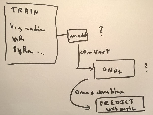
ONNX on random forest#
NbImage("process.png", width=500)
rf
RandomForestRegressor(n_estimators=10)
Conversion to ONNX#
from skl2onnx import convert_sklearn
from skl2onnx.common.data_types import FloatTensorType
model_onnx = convert_sklearn(rf, "rf_diabetes",
                             [('input', FloatTensorType([1, 10]))])
print(str(model_onnx)[:450] + "\n...")
ir_version: 6
producer_name: "skl2onnx"
producer_version: "1.7.0"
domain: "ai.onnx"
model_version: 0
doc_string: ""
graph {
  node {
    input: "input"
    output: "variable"
    name: "TreeEnsembleRegressor"
    op_type: "TreeEnsembleRegressor"
    attribute {
      name: "n_targets"
      i: 1
      type: INT
    }
    attribute {
      name: "nodes_falsenodeids"
      ints: 324
      ints: 243
      ints: 146
      ints: 105
      ints: 62
...
Save the model#
with open('rf_sklearn.onnx', "wb") as f:
    f.write(model_onnx.SerializeToString())
Compute predictions#
import onnxruntime

sess = onnxruntime.InferenceSession("rf_sklearn.onnx")

for i in sess.get_inputs():
    print('Input:', i)
for o in sess.get_outputs():
    print('Output:', o)
Input: NodeArg(name='input', type='tensor(float)', shape=[1, 10])
Output: NodeArg(name='variable', type='tensor(float)', shape=[1, 1])
import numpy

def predict_onnxrt(x):
    return sess.run(["variable"], {'input': x})

print("Prediction:", predict_onnxrt(diabetes_X_test[:1].astype(numpy.float32)))
Prediction: [array([[177.40001]], dtype=float32)]
measures_rf += [timeexec("onnx", "predict_onnxrt(diabetes_X_test[:1].astype(numpy.float32))",
                         context=globals())]
Average: 18.94 µs deviation 11.57 µs (with 50 runs) in [12.18 µs, 43.00 µs]
fig, ax = plt.subplots(1, 1, figsize=(10,3))
df = pandas.DataFrame(data=measures_rf)
df = df.set_index("legend").sort_values("average")
df[["average", "deviation"]].plot(kind="barh", logx=True, ax=ax, xerr="deviation",
                                  legend=False, fontsize=12, width=0.8)
ax.set_ylabel("")
ax.grid(b=True, which="major")
ax.grid(b=True, which="minor")
ax.set_title("Prediction time for one observation\nRandom Forest (10 trees)");
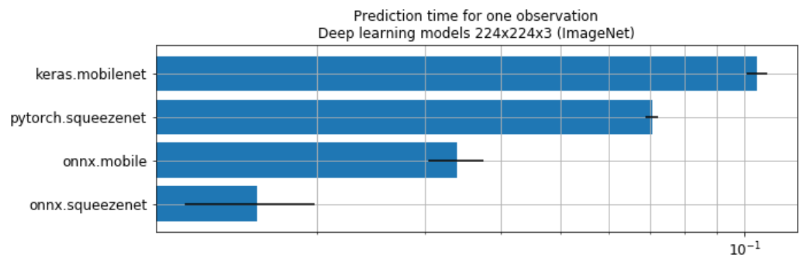
Deep learning#
transfer learning with keras
orther convert pytorch, caffee…
Code is available at MS Experience 2018.
Perf#
NbImage("dlpref.png", width=600)
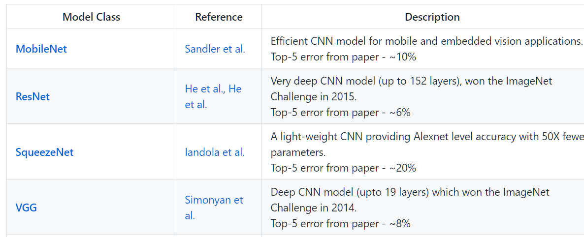
Model zoo#
NbImage("zoo.png", width=800)
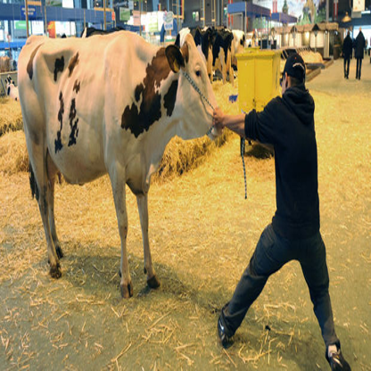
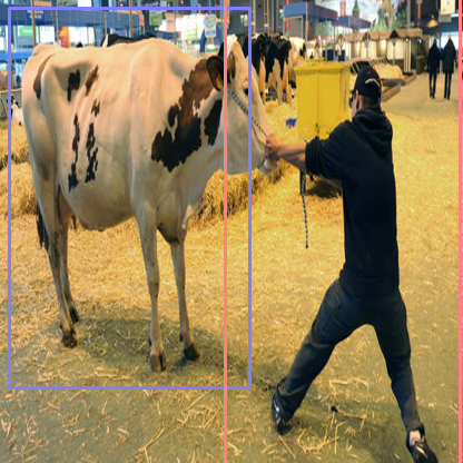
Tiny yolo#
Source: TinyYOLOv2 on onnx
from pyensae.datasource import download_data
download_data("tiny_yolov2.tar.gz",
              url="https://onnxzoo.blob.core.windows.net/models/opset_8/tiny_yolov2/")
['.\tiny_yolov2/./Model.onnx',
 '.\tiny_yolov2/./test_data_set_2/input_0.pb',
 '.\tiny_yolov2/./test_data_set_2/output_0.pb',
 '.\tiny_yolov2/./test_data_set_1/input_0.pb',
 '.\tiny_yolov2/./test_data_set_1/output_0.pb',
 '.\tiny_yolov2/./test_data_set_0/input_0.pb',
 '.\tiny_yolov2/./test_data_set_0/output_0.pb']
sess = onnxruntime.InferenceSession("tiny_yolov2/Model.onnx")
for i in sess.get_inputs():
    print('Input:', i)
for o in sess.get_outputs():
    print('Output:', o)
Input: NodeArg(name='image', type='tensor(float)', shape=['None', 3, 416, 416])
Output: NodeArg(name='grid', type='tensor(float)', shape=['None', 125, 13, 13])
from PIL import Image,ImageDraw
img = Image.open('Au-Salon-de-l-agriculture-la-campagne-recrute.jpg')
img

img2 = img.resize((416, 416))
img2
X = numpy.asarray(img2)
X = X.transpose(2,0,1)
X = X.reshape(1,3,416,416)

out = sess.run(None, {'image': X.astype(numpy.float32)})
out = out[0][0]
def display_yolo(img, seuil):
    import numpy as np
    numClasses = 20
    anchors = [1.08, 1.19, 3.42, 4.41, 6.63, 11.38, 9.42, 5.11, 16.62, 10.52]

    def sigmoid(x, derivative=False):
        return x*(1-x) if derivative else 1/(1+np.exp(-x))

    def softmax(x):
        scoreMatExp = np.exp(np.asarray(x))
        return scoreMatExp / scoreMatExp.sum(0)

    clut = [(0,0,0),(255,0,0),(255,0,255),(0,0,255),(0,255,0),(0,255,128),
            (128,255,0),(128,128,0),(0,128,255),(128,0,128),
            (255,0,128),(128,0,255),(255,128,128),(128,255,128),(255,255,0),
            (255,128,128),(128,128,255),(255,128,128),(128,255,128),(128,255,128)]
    label = ["aeroplane","bicycle","bird","boat","bottle",
             "bus","car","cat","chair","cow","diningtable",
             "dog","horse","motorbike","person","pottedplant",
             "sheep","sofa","train","tvmonitor"]

    draw = ImageDraw.Draw(img)
    for cy in range(0,13):
        for cx in range(0,13):
            for b in range(0,5):
                channel = b*(numClasses+5)
                tx = out[channel  ][cy][cx]
                ty = out[channel+1][cy][cx]
                tw = out[channel+2][cy][cx]
                th = out[channel+3][cy][cx]
                tc = out[channel+4][cy][cx]

                x = (float(cx) + sigmoid(tx))*32
                y = (float(cy) + sigmoid(ty))*32

                w = np.exp(tw) * 32 * anchors[2*b  ]
                h = np.exp(th) * 32 * anchors[2*b+1]

                confidence = sigmoid(tc)

                classes = np.zeros(numClasses)
                for c in range(0,numClasses):
                    classes[c] = out[channel + 5 +c][cy][cx]
                    classes = softmax(classes)
                detectedClass = classes.argmax()

                if seuil < classes[detectedClass]*confidence:
                    color =clut[detectedClass]
                    x = x - w/2
                    y = y - h/2
                    draw.line((x  ,y  ,x+w,y ),fill=color, width=3)
                    draw.line((x  ,y  ,x  ,y+h),fill=color, width=3)
                    draw.line((x+w,y  ,x+w,y+h),fill=color, width=3)
                    draw.line((x  ,y+h,x+w,y+h),fill=color, width=3)

    return img
img2 = img.resize((416, 416))
display_yolo(img2, 0.038)
Conclusion#
ONNX is a working progress, active development
ONNX is open source
ONNX does not depend on the machine learning framework
ONNX provides dedicated runtimes
ONNX is fast and available in Python…
Metadata to trace deployed models
meta = sess.get_modelmeta()
meta.description
"The Tiny YOLO network from the paper 'YOLO9000: Better, Faster, Stronger' (2016), arXiv:1612.08242"
meta.producer_name, meta.version
('OnnxMLTools', 0)