Session 26/6/2017 - machine learning#
Links: notebook, html, PDF, python, slides, GitHub
Découverte des trois problèmes de machine learning exposé dans l’article Machine Learning - session 6.
from jyquickhelper import add_notebook_menu
add_notebook_menu()
Problème 1 : comparaison random forest, linéaire#
C’est un problème de régression. On cherche à comparer une random forest avec un modèle linéaire.
Comparaison des tests de coefficients pour un modèle linéaire OLS et des features importance
Résultat au niveau d’une observation treeinterpreter
Données : Housing, Forest Fire
Données#
import pandas
df = pandas.read_csv("data/housing.data", delim_whitespace=True, header=None)
df.head()
| 0 | 1 | 2 | 3 | 4 | 5 | 6 | 7 | 8 | 9 | 10 | 11 | 12 | 13 | |
|---|---|---|---|---|---|---|---|---|---|---|---|---|---|---|
| 0 | 0.00632 | 18.0 | 2.31 | 0 | 0.538 | 6.575 | 65.2 | 4.0900 | 1 | 296.0 | 15.3 | 396.90 | 4.98 | 24.0 |
| 1 | 0.02731 | 0.0 | 7.07 | 0 | 0.469 | 6.421 | 78.9 | 4.9671 | 2 | 242.0 | 17.8 | 396.90 | 9.14 | 21.6 |
| 2 | 0.02729 | 0.0 | 7.07 | 0 | 0.469 | 7.185 | 61.1 | 4.9671 | 2 | 242.0 | 17.8 | 392.83 | 4.03 | 34.7 |
| 3 | 0.03237 | 0.0 | 2.18 | 0 | 0.458 | 6.998 | 45.8 | 6.0622 | 3 | 222.0 | 18.7 | 394.63 | 2.94 | 33.4 |
| 4 | 0.06905 | 0.0 | 2.18 | 0 | 0.458 | 7.147 | 54.2 | 6.0622 | 3 | 222.0 | 18.7 | 396.90 | 5.33 | 36.2 |
cols = "CRIM ZN INDUS CHAS NOX RM AGE DIS RAD TAX PTRATIO B LSTAT MEDV".split()
df.columns = cols
df.head()
| CRIM | ZN | INDUS | CHAS | NOX | RM | AGE | DIS | RAD | TAX | PTRATIO | B | LSTAT | MEDV | |
|---|---|---|---|---|---|---|---|---|---|---|---|---|---|---|
| 0 | 0.00632 | 18.0 | 2.31 | 0 | 0.538 | 6.575 | 65.2 | 4.0900 | 1 | 296.0 | 15.3 | 396.90 | 4.98 | 24.0 |
| 1 | 0.02731 | 0.0 | 7.07 | 0 | 0.469 | 6.421 | 78.9 | 4.9671 | 2 | 242.0 | 17.8 | 396.90 | 9.14 | 21.6 |
| 2 | 0.02729 | 0.0 | 7.07 | 0 | 0.469 | 7.185 | 61.1 | 4.9671 | 2 | 242.0 | 17.8 | 392.83 | 4.03 | 34.7 |
| 3 | 0.03237 | 0.0 | 2.18 | 0 | 0.458 | 6.998 | 45.8 | 6.0622 | 3 | 222.0 | 18.7 | 394.63 | 2.94 | 33.4 |
| 4 | 0.06905 | 0.0 | 2.18 | 0 | 0.458 | 7.147 | 54.2 | 6.0622 | 3 | 222.0 | 18.7 | 396.90 | 5.33 | 36.2 |
X = df.drop("MEDV", axis=1)
y = df["MEDV"]
from sklearn.model_selection import train_test_split
X_train, X_test, y_train, y_test = train_test_split(X, y, test_size=0.33)
Random Forest#
from sklearn.ensemble import RandomForestRegressor
clr = RandomForestRegressor()
clr.fit(X, y)
RandomForestRegressor(bootstrap=True, criterion='mse', max_depth=None,
                      max_features='auto', max_leaf_nodes=None,
                      min_impurity_decrease=0.0, min_impurity_split=None,
                      min_samples_leaf=1, min_samples_split=2,
                      min_weight_fraction_leaf=0.0, n_estimators=100,
                      n_jobs=None, oob_score=False, random_state=None,
                      verbose=0, warm_start=False)
importances = clr.feature_importances_
importances
array([0.04377988, 0.00098713, 0.00669368, 0.00092023, 0.02074126,
       0.4076033 , 0.01283279, 0.06458251, 0.0036521 , 0.01366027,
       0.01576497, 0.01209152, 0.39669034])
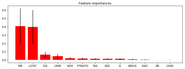
On s’inspire de l’exemple Feature importances with forests of trees.
%matplotlib inline
import matplotlib.pyplot as plt
import numpy as np
plt.figure(figsize=(12,4))
indices = np.argsort(importances)[::-1]
std = np.std([tree.feature_importances_ for tree in clr.estimators_],
             axis=0)
plt.title("Feature importances")
plt.bar(range(X.shape[1]), importances[indices],
        color="r", yerr=std[indices], align="center")
xlabels = list(df.columns[:-1])
xlabels = [xlabels[i] for i in indices]
plt.xticks(range(X.shape[1]), xlabels)
plt.xlim([-1, X.shape[1]])
plt.show()
from sklearn.metrics import r2_score
r2_score(y_train, clr.predict(X_train))
0.979236135448983
r2_score(y_test, clr.predict(X_test))
0.9843720628811461
Modèle linéaire#
import statsmodels.api as sm
model = sm.OLS(y_train, X_train)
results = model.fit()
results.params
CRIM      -0.109867
ZN         0.045855
INDUS     -0.054801
CHAS       3.758792
NOX       -5.285538
RM         6.267853
AGE       -0.022554
DIS       -1.169496
RAD        0.221785
TAX       -0.010410
PTRATIO   -0.447963
B          0.016474
LSTAT     -0.259210
dtype: float64
results.summary()
| Dep. Variable: | MEDV | R-squared: | 0.958 |
|---|---|---|---|
| Model: | OLS | Adj. R-squared: | 0.957 |
| Method: | Least Squares | F-statistic: | 575.3 |
| Date: | Fri, 07 Jun 2019 | Prob (F-statistic): | 7.10e-216 |
| Time: | 16:38:39 | Log-Likelihood: | -1025.5 |
| No. Observations: | 339 | AIC: | 2077. |
| Df Residuals: | 326 | BIC: | 2127. |
| Df Model: | 13 | ||
| Covariance Type: | nonrobust |
| coef | std err | t | P>|t| | [0.025 | 0.975] | |
|---|---|---|---|---|---|---|
| CRIM | -0.1099 | 0.039 | -2.845 | 0.005 | -0.186 | -0.034 |
| ZN | 0.0459 | 0.018 | 2.543 | 0.011 | 0.010 | 0.081 |
| INDUS | -0.0548 | 0.079 | -0.697 | 0.486 | -0.209 | 0.100 |
| CHAS | 3.7588 | 1.116 | 3.370 | 0.001 | 1.564 | 5.953 |
| NOX | -5.2855 | 4.398 | -1.202 | 0.230 | -13.938 | 3.367 |
| RM | 6.2679 | 0.405 | 15.461 | 0.000 | 5.470 | 7.065 |
| AGE | -0.0226 | 0.017 | -1.325 | 0.186 | -0.056 | 0.011 |
| DIS | -1.1695 | 0.249 | -4.692 | 0.000 | -1.660 | -0.679 |
| RAD | 0.2218 | 0.083 | 2.672 | 0.008 | 0.058 | 0.385 |
| TAX | -0.0104 | 0.005 | -2.155 | 0.032 | -0.020 | -0.001 |
| PTRATIO | -0.4480 | 0.137 | -3.261 | 0.001 | -0.718 | -0.178 |
| B | 0.0165 | 0.003 | 4.767 | 0.000 | 0.010 | 0.023 |
| LSTAT | -0.2592 | 0.065 | -3.959 | 0.000 | -0.388 | -0.130 |
| Omnibus: | 170.276 | Durbin-Watson: | 1.981 |
|---|---|---|---|
| Prob(Omnibus): | 0.000 | Jarque-Bera (JB): | 1726.398 |
| Skew: | 1.839 | Prob(JB): | 0.00 |
| Kurtosis: | 13.426 | Cond. No. | 8.91e+03 |
Warnings:
[1] Standard Errors assume that the covariance matrix of the errors is correctly specified.
[2] The condition number is large, 8.91e+03. This might indicate that there are
strong multicollinearity or other numerical problems.
model = sm.OLS(y,X.drop("LSTAT", axis=1))
results = model.fit()
results.summary()
| Dep. Variable: | MEDV | R-squared: | 0.954 |
|---|---|---|---|
| Model: | OLS | Adj. R-squared: | 0.953 |
| Method: | Least Squares | F-statistic: | 846.6 |
| Date: | Fri, 07 Jun 2019 | Prob (F-statistic): | 2.38e-320 |
| Time: | 16:38:39 | Log-Likelihood: | -1556.1 |
| No. Observations: | 506 | AIC: | 3136. |
| Df Residuals: | 494 | BIC: | 3187. |
| Df Model: | 12 | ||
| Covariance Type: | nonrobust |
| coef | std err | t | P>|t| | [0.025 | 0.975] | |
|---|---|---|---|---|---|---|
| CRIM | -0.1439 | 0.036 | -3.990 | 0.000 | -0.215 | -0.073 |
| ZN | 0.0413 | 0.015 | 2.696 | 0.007 | 0.011 | 0.071 |
| INDUS | -0.0370 | 0.068 | -0.540 | 0.589 | -0.172 | 0.098 |
| CHAS | 3.2525 | 0.961 | 3.384 | 0.001 | 1.364 | 5.141 |
| NOX | -10.8653 | 3.422 | -3.175 | 0.002 | -17.590 | -4.141 |
| RM | 7.1436 | 0.289 | 24.734 | 0.000 | 6.576 | 7.711 |
| AGE | -0.0449 | 0.014 | -3.235 | 0.001 | -0.072 | -0.018 |
| DIS | -1.2292 | 0.206 | -5.980 | 0.000 | -1.633 | -0.825 |
| RAD | 0.2008 | 0.071 | 2.829 | 0.005 | 0.061 | 0.340 |
| TAX | -0.0100 | 0.004 | -2.391 | 0.017 | -0.018 | -0.002 |
| PTRATIO | -0.6575 | 0.112 | -5.881 | 0.000 | -0.877 | -0.438 |
| B | 0.0165 | 0.003 | 5.779 | 0.000 | 0.011 | 0.022 |
| Omnibus: | 277.013 | Durbin-Watson: | 0.927 |
|---|---|---|---|
| Prob(Omnibus): | 0.000 | Jarque-Bera (JB): | 3084.310 |
| Skew: | 2.148 | Prob(JB): | 0.00 |
| Kurtosis: | 14.307 | Cond. No. | 8.13e+03 |
Warnings:
[1] Standard Errors assume that the covariance matrix of the errors is correctly specified.
[2] The condition number is large, 8.13e+03. This might indicate that there are
strong multicollinearity or other numerical problems.
TPOT#
TPOT est un module d’apprentissage automatique.
try:
    from tpot import TPOTRegressor
except ImportError:
    # for sklearn 0.22
    import sklearn.preprocessing
    from sklearn.impute import SimpleImputer
    sklearn.preprocessing.Imputer = SimpleImputer
    from tpot import TPOTRegressor

tpot = TPOTRegressor(generations=2, population_size=50, verbosity=2)
tpot.fit(X_train, y_train)
print(tpot.score(X_test, y_test))
tpot.export('tpot_boston_pipeline.py')
HBox(children=(IntProgress(value=0, description='Optimization Progress', max=150, style=ProgressStyle(descript…
Generation 1 - Current best internal CV score: -10.19955600172555
Generation 2 - Current best internal CV score: -10.19955600172555

Best pipeline: XGBRegressor(StandardScaler(input_matrix), learning_rate=0.1, max_depth=9, min_child_weight=2, n_estimators=100, nthread=1, subsample=0.8)
-9.01100125963658
Le module optimise les hyperparamètres, parfois un peu trop à en juger la mauvaise performance obtenue sur la base de test.
r2_score(y_train, tpot.predict(X_train))
0.9994364901579464
r2_score(y_test, tpot.predict(X_test))
0.8978805496355459
Feature importance pour une observations#
On reprend la première random forest et on utilise le module treeinterpreter.
clr = RandomForestRegressor()
clr.fit(X, y)
RandomForestRegressor(bootstrap=True, criterion='mse', max_depth=None,
                      max_features='auto', max_leaf_nodes=None,
                      min_impurity_decrease=0.0, min_impurity_split=None,
                      min_samples_leaf=1, min_samples_split=2,
                      min_weight_fraction_leaf=0.0, n_estimators=100,
                      n_jobs=None, oob_score=False, random_state=None,
                      verbose=0, warm_start=False)
from treeinterpreter import treeinterpreter as ti
prediction, bias, contributions = ti.predict(clr, X_test)
for i in range(min(2, X_train.shape[0])):
    print("Instance", i)
    print("Bias (trainset mean)", bias[i])
    print("Feature contributions:")
    for c, feature in sorted(zip(contributions[i], df.columns),
                             key=lambda x: -abs(x[0])):
        print(feature, round(c, 2))
    print( "-"*20)
Instance 0
Bias (trainset mean) 22.527195652173905
Feature contributions:
RM 7.53
LSTAT 1.58
TAX -0.64
PTRATIO 0.6
DIS -0.4
INDUS 0.19
RAD -0.18
AGE 0.13
ZN 0.12
CRIM 0.07
NOX 0.06
B -0.01
CHAS -0.01
--------------------
Instance 1
Bias (trainset mean) 22.527195652173905
Feature contributions:
LSTAT -5.04
RM -1.64
B -0.9
NOX -0.89
CRIM -0.81
DIS 0.64
AGE 0.17
PTRATIO -0.07
TAX -0.04
CHAS -0.02
INDUS -0.0
ZN 0.0
RAD 0.0
--------------------
Problème 2 : série temporelle#
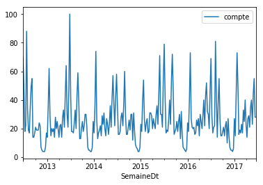
On prend une série sur Google Trends, dans notre cas, c’est la requête tennis live. On compare une approche linéaire et une approche non linéaire.
Approche linéaire#
import pandas
df = pandas.read_csv("data/multiTimeline.csv", skiprows=1)
df.columns= ["Semaine", "compte"]
df["SemaineDt"] = pandas.to_datetime(df.Semaine)
df=df.set_index("SemaineDt")
df["compte"] = df["compte"].astype(float)
df.head()
| Semaine | compte | |
|---|---|---|
| SemaineDt | ||
| 2012-07-01 | 2012-07-01 | 70.0 |
| 2012-07-08 | 2012-07-08 | 49.0 |
| 2012-07-15 | 2012-07-15 | 18.0 |
| 2012-07-22 | 2012-07-22 | 22.0 |
| 2012-07-29 | 2012-07-29 | 88.0 |
%matplotlib inline
df.plot()
<matplotlib.axes._subplots.AxesSubplot at 0x19c15163358>
from statsmodels.tsa.arima_model import ARIMA
arma_mod = ARIMA(df["compte"].values, order=(6 ,1, 1))
res = arma_mod.fit()
res.params
array([ 0.00418581,  0.59035757, -0.32540695,  0.23286807, -0.03300838,
        0.06434307, -0.07204017, -0.99999983])
res.summary()
| Dep. Variable: | D.y | No. Observations: | 259 |
|---|---|---|---|
| Model: | ARIMA(6, 1, 1) | Log Likelihood | -1055.581 |
| Method: | css-mle | S.D. of innovations | 14.116 |
| Date: | Fri, 07 Jun 2019 | AIC | 2129.161 |
| Time: | 16:45:54 | BIC | 2161.173 |
| Sample: | 1 | HQIC | 2142.032 |
| coef | std err | z | P>|z| | [0.025 | 0.975] | |
|---|---|---|---|---|---|---|
| const | 0.0042 | 0.021 | 0.196 | 0.845 | -0.038 | 0.046 |
| ar.L1.D.y | 0.5904 | 0.063 | 9.431 | 0.000 | 0.468 | 0.713 |
| ar.L2.D.y | -0.3254 | 0.072 | -4.507 | 0.000 | -0.467 | -0.184 |
| ar.L3.D.y | 0.2329 | 0.075 | 3.097 | 0.002 | 0.085 | 0.380 |
| ar.L4.D.y | -0.0330 | 0.076 | -0.433 | 0.665 | -0.182 | 0.116 |
| ar.L5.D.y | 0.0643 | 0.076 | 0.842 | 0.400 | -0.085 | 0.214 |
| ar.L6.D.y | -0.0720 | 0.066 | -1.096 | 0.274 | -0.201 | 0.057 |
| ma.L1.D.y | -1.0000 | 0.010 | -96.075 | 0.000 | -1.020 | -0.980 |
| Real | Imaginary | Modulus | Frequency | |
|---|---|---|---|---|
| AR.1 | -1.2011 | -1.2144j | 1.7080 | -0.3741 |
| AR.2 | -1.2011 | +1.2144j | 1.7080 | 0.3741 |
| AR.3 | 0.1840 | -1.4018j | 1.4138 | -0.2292 |
| AR.4 | 0.1840 | +1.4018j | 1.4138 | 0.2292 |
| AR.5 | 1.4636 | -0.4882j | 1.5429 | -0.0512 |
| AR.6 | 1.4636 | +0.4882j | 1.5429 | 0.0512 |
| MA.1 | 1.0000 | +0.0000j | 1.0000 | 0.0000 |
Méthode non linéaire#
On construire la matrice des séries décalées. Cette méthode permet de sortir du cadre linéaire et d’ajouter d’autres variables.
from statsmodels.tsa.tsatools import lagmat
lag = 8
X = lagmat(df["compte"], lag)
lagged = df.copy()
for c in range(1,lag+1):
    lagged["lag%d" % c] = X[:, c-1]
pandas.concat([lagged.head(), lagged.tail()])
| Semaine | compte | lag1 | lag2 | lag3 | lag4 | lag5 | lag6 | lag7 | lag8 | |
|---|---|---|---|---|---|---|---|---|---|---|
| SemaineDt | ||||||||||
| 2012-07-01 | 2012-07-01 | 70.0 | 0.0 | 0.0 | 0.0 | 0.0 | 0.0 | 0.0 | 0.0 | 0.0 |
| 2012-07-08 | 2012-07-08 | 49.0 | 70.0 | 0.0 | 0.0 | 0.0 | 0.0 | 0.0 | 0.0 | 0.0 |
| 2012-07-15 | 2012-07-15 | 18.0 | 49.0 | 70.0 | 0.0 | 0.0 | 0.0 | 0.0 | 0.0 | 0.0 |
| 2012-07-22 | 2012-07-22 | 22.0 | 18.0 | 49.0 | 70.0 | 0.0 | 0.0 | 0.0 | 0.0 | 0.0 |
| 2012-07-29 | 2012-07-29 | 88.0 | 22.0 | 18.0 | 49.0 | 70.0 | 0.0 | 0.0 | 0.0 | 0.0 |
| 2017-05-21 | 2017-05-21 | 23.0 | 40.0 | 35.0 | 21.0 | 29.0 | 27.0 | 14.0 | 23.0 | 40.0 |
| 2017-05-28 | 2017-05-28 | 44.0 | 23.0 | 40.0 | 35.0 | 21.0 | 29.0 | 27.0 | 14.0 | 23.0 |
| 2017-06-04 | 2017-06-04 | 55.0 | 44.0 | 23.0 | 40.0 | 35.0 | 21.0 | 29.0 | 27.0 | 14.0 |
| 2017-06-11 | 2017-06-11 | 28.0 | 55.0 | 44.0 | 23.0 | 40.0 | 35.0 | 21.0 | 29.0 | 27.0 |
| 2017-06-18 | 2017-06-18 | 28.0 | 28.0 | 55.0 | 44.0 | 23.0 | 40.0 | 35.0 | 21.0 | 29.0 |
xc = ["lag%d" % i for i in range(1,lag+1)]
split = 0.66
isplit = int(len(lagged) * split)
xt = lagged[10:][xc]
yt = lagged[10:]["compte"]
X_train, y_train, X_test, y_test = xt[:isplit], yt[:isplit], xt[isplit:], yt[isplit:]
from sklearn.ensemble import RandomForestRegressor
clr = RandomForestRegressor()
clr.fit(X_train, y_train)
RandomForestRegressor(bootstrap=True, criterion='mse', max_depth=None,
                      max_features='auto', max_leaf_nodes=None,
                      min_impurity_decrease=0.0, min_impurity_split=None,
                      min_samples_leaf=1, min_samples_split=2,
                      min_weight_fraction_leaf=0.0, n_estimators=100,
                      n_jobs=None, oob_score=False, random_state=None,
                      verbose=0, warm_start=False)
from sklearn.metrics import r2_score
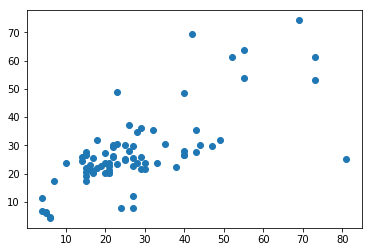
r2 = r2_score(y_test.values, clr.predict(X_test))
r2
0.4878325848907805
plt.scatter(y_test.values, clr.predict(X_test));
<matplotlib.collections.PathCollection at 0x19c26b9a2e8>
Texte#
On cherche à comparer une LDA avec word2vec et kmeans et les données qui sont sur ensae_teaching_cs/src/ensae_teaching_cs/data/data_web/.
from ensae_teaching_cs.data import twitter_zip
df = twitter_zip(as_df=True)
df.head(n=2).T
| 0 | 1 | |
|---|---|---|
| index | 776066992054861825 | 776067660979245056 |
| nb_user_mentions | 0 | 0 |
| nb_extended_entities | 0 | 0 |
| nb_hashtags | 1 | 1 |
| geo | NaN | NaN |
| text_hashtags | , SiJétaisPrésident | , SiJétaisPrésident |
| annee | 2016 | 2016 |
| delimit_mention | NaN | NaN |
| lang | fr | fr |
| id_str | 7.76067e+17 | 7.76068e+17 |
| text_mention | NaN | NaN |
| retweet_count | 4 | 5 |
| favorite_count | 3 | 8 |
| type_extended_entities | [] | [] |
| text | #SiJétaisPrésident se serait la fin du monde..... | #SiJétaisPrésident je donnerai plus de vacance... |
| nb_user_photos | 0 | 0 |
| nb_urls | 0 | 0 |
| nb_symbols | 0 | 0 |
| created_at | Wed Sep 14 14:36:04 +0000 2016 | Wed Sep 14 14:38:43 +0000 2016 |
| delimit_hash | , 0, 18 | , 0, 18 |
Des mots aux coordonnées - tf-idf#
keep = df.text.dropna().index
dfnonan = df.iloc[keep, :]
dfnonan.shape
(5087, 20)
from sklearn.feature_extraction.text import TfidfVectorizer
tfidf_vectorizer = TfidfVectorizer(max_df=0.95, min_df=2, max_features=1000)
tfidf = tfidf_vectorizer.fit_transform(dfnonan["text"])
tfidf[:2, :]
<2x1000 sparse matrix of type '<class 'numpy.float64'>'
    with 21 stored elements in Compressed Sparse Row format>
tfidf[:2, :].todense()
matrix([[0., 0., 0., ..., 0., 0., 0.],
        [0., 0., 0., ..., 0., 0., 0.]])
LDA#
from sklearn.decomposition import LatentDirichletAllocation
lda = LatentDirichletAllocation(n_components=10, max_iter=5,
                                learning_method='online',
                                learning_offset=50.,
                                random_state=0)
lda.fit(tfidf)
LatentDirichletAllocation(batch_size=128, doc_topic_prior=None,
                          evaluate_every=-1, learning_decay=0.7,
                          learning_method='online', learning_offset=50.0,
                          max_doc_update_iter=100, max_iter=5,
                          mean_change_tol=0.001, n_components=10, n_jobs=None,
                          perp_tol=0.1, random_state=0, topic_word_prior=None,
                          total_samples=1000000.0, verbose=0)
tf_feature_names = tfidf_vectorizer.get_feature_names()
tf_feature_names[100:103]
['avoir', 'bac', 'bah']
lda.components_.shape
(10, 1000)
On obtient dix vecteurs qui représentent les dix vecteurs associés aux dix clusters. Chaque dimension relié au fait que le mot appartient ou non au cluster.
def print_top_words(model, feature_names, n_top_words):
    for topic_idx, topic in enumerate(model.components_):
        print("Topic #%d:" % topic_idx)
        print(" ".join([feature_names[i]
                        for i in topic.argsort()[:-n_top_words - 1:-1]]))
    print()
print_top_words(lda, tf_feature_names, 10)
Topic #0:
gratuit mcdo supprimerai école soir kebab macdo kfc domicile cc
Topic #1:
macron co https de la est le il et hollande
Topic #2:
sijetaispresident je les de la et le des en pour
Topic #3:
notaires eu organiserais mets carte nouveaux journées installation cache créer
Topic #4:
sijetaispresident interdirais les je ballerines la serait serais bah de
Topic #5:
ministre de sijetaispresident la je premier mort et nommerais président
Topic #6:
cours le supprimerais jour sijetaispresident lundi samedi semaine je vendredi
Topic #7:
port interdirait démissionnerais promesses heure rendrai ballerine mes changement christineboutin
Topic #8:
seraient sijetaispresident gratuits aux les nos putain éducation nationale bonne
Topic #9:
bordel seront légaliserai putes gratuites pizza mot virerais vitesse dutreil
Clustering#
from sklearn.cluster import KMeans
km = KMeans(n_clusters=10)
km.fit(tfidf)
KMeans(algorithm='auto', copy_x=True, init='k-means++', max_iter=300,
       n_clusters=10, n_init=10, n_jobs=None, precompute_distances='auto',
       random_state=None, tol=0.0001, verbose=0)
km.cluster_centers_.shape
(10, 1000)
def print_top_words(model, feature_names, n_top_words):
    for topic_idx, topic in enumerate(model.cluster_centers_):
        print("Topic #%d:" % topic_idx)
        print(" ".join([feature_names[i]
                        for i in topic.argsort()[:-n_top_words - 1:-1]]))
    print()
print_top_words(km, tf_feature_names, 10)
Topic #0:
ferais je sijetaispresident les en sorte que de et un
Topic #1:
le sijetaispresident je monde et pour de tout des les
Topic #2:
de sijetaispresident la en et des une un plus aurait
Topic #3:
https co macron de la le les via et sijetaispresident
Topic #4:
les sijetaispresident je de et tous des seraient pour ballerines
Topic #5:
serait sijetaispresident la le merde de ça et on dans
Topic #6:
je sijetaispresident la des me et ferai pas en au
Topic #7:
macron est il de pas la hollande le gauche que
Topic #8:
ministre premier nommerais sijetaispresident de je la mickey serait nommerai
Topic #9:
serais je sijetaispresident un pas ne président que la de
Ah les stop words….