Custom DecisionTreeRegressor adapted to a linear regression

Links: notebook, html, PDF, python, slides, GitHub

A DecisionTreeRegressor can be trained with a couple of possible criterions but it is possible to implement a custom one (see hellinger_distance_criterion). See also tutorial Cython example of exposing C-computed arrays in Python without data copies which describes a way to implement fast cython extensions.

from jyquickhelper import add_notebook_menu
add_notebook_menu()

%matplotlib inline

import warnings
warnings.simplefilter("ignore")

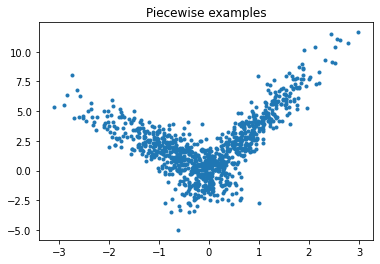
Piecewise data

Let’s build a toy problem based on two linear models.

import numpy
import numpy.random as npr
X = npr.normal(size=(1000,4))
alpha = [4, -2]
t = (X[:, 0] + X[:, 3] * 0.5) > 0
switch = numpy.zeros(X.shape[0])
switch[t] = 1
y = alpha[0] * X[:, 0] * t + alpha[1] * X[:, 0] * (1-t) + X[:, 2]

import matplotlib.pyplot as plt
fig, ax = plt.subplots(1, 1)
ax.plot(X[:, 0], y, ".")
ax.set_title("Piecewise examples");

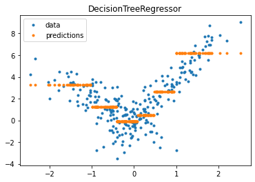
DecisionTreeRegressor

from sklearn.model_selection import train_test_split
X_train, X_test, y_train, y_test = train_test_split(X[:, :1], y)

from sklearn.tree import DecisionTreeRegressor

model = DecisionTreeRegressor(min_samples_leaf=100)
model.fit(X_train, y_train)

DecisionTreeRegressor(min_samples_leaf=100)

pred = model.predict(X_test)
pred[:5]

array([ 3.29436256,  0.50924806, -0.07129149,  0.50924806,  2.64957806])

fig, ax = plt.subplots(1, 1)
ax.plot(X_test[:, 0], y_test, ".", label='data')
ax.plot(X_test[:, 0], pred, ".", label="predictions")
ax.set_title("DecisionTreeRegressor")
ax.legend();

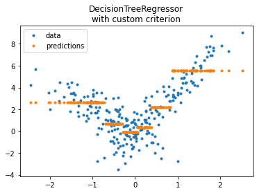
DecisionTreeRegressor with custom implementation

import sklearn
from pyquickhelper.texthelper import compare_module_version
if compare_module_version(sklearn.__version__, '0.21') < 0:
    print("Next step requires scikit-learn >= 0.21")
else:
    print("sklearn.__version__ =", sklearn.__version__)

sklearn.__version__ = 1.1.dev0

from mlinsights.mlmodel.piecewise_tree_regression_criterion import SimpleRegressorCriterion

model2 = DecisionTreeRegressor(min_samples_leaf=100,
                              criterion=SimpleRegressorCriterion(X_train))
model2.fit(X_train, y_train)

DecisionTreeRegressor(criterion=<mlinsights.mlmodel.piecewise_tree_regression_criterion.SimpleRegressorCriterion object at 0x000001FC680A0BF0>,
                      min_samples_leaf=100)

pred = model2.predict(X_test)
pred[:5]

array([ 2.65757699,  0.37665413, -0.07967816,  0.37665413,  5.57229226])

fig, ax = plt.subplots(1, 1)
ax.plot(X_test[:, 0], y_test, ".", label='data')
ax.plot(X_test[:, 0], pred, ".", label="predictions")
ax.set_title("DecisionTreeRegressor\nwith custom criterion")
ax.legend();

Computation time

The custom criterion is not really efficient but it was meant that way. The code can be found in piecewise_tree_regression_criterion. Bascially, it is slow because each time the algorithm optimizing the tree needs the class Criterion to evaluate the impurity reduction for a split, the computation happens on the whole data under the node being split. The implementation in _criterion.pyx does it once.

%timeit model.fit(X_train, y_train)

551 µs ± 93.7 µs per loop (mean ± std. dev. of 7 runs, 1000 loops each)

%timeit model2.fit(X_train, y_train)

43.9 ms ± 2.21 ms per loop (mean ± std. dev. of 7 runs, 10 loops each)

A loop is involved every time the criterion of the node is involved which raises a the computation cost of lot. The method _mse is called each time the algorithm training the decision tree needs to evaluate a cut, one cut involves elements betwee, position [start, end[.

cdef void _mean(self, SIZE_t start, SIZE_t end, DOUBLE_t *mean, DOUBLE_t *weight) nogil:

if start == end:

mean[0] = 0. return

cdef DOUBLE_t m = 0. cdef DOUBLE_t w = 0. cdef int k for k in range(start, end):

m += self.sample_wy[k] w += self.sample_w[k]

weight[0] = w mean[0] = 0. if w == 0. else m / w

cdef double _mse(self, SIZE_t start, SIZE_t end, DOUBLE_t mean, DOUBLE_t weight) nogil:

if start == end:

return 0.

cdef DOUBLE_t squ = 0. cdef int k for k in range(start, end):

squ += (self.y[self.sample_i[k], 0] - mean) ** 2 * self.sample_w[k]

return 0. if weight == 0. else squ / weight

Better implementation

I rewrote my first implementation to be closer to what scikit-learn is doing. The criterion is computed once for all possible cut and then retrieved on demand. The code is below, arrays sample_wy_left is the cumulated sum of starting from the left side (lower Y). The loop disappeared.

cdef void _mean(self, SIZE_t start, SIZE_t end, DOUBLE_t *mean, DOUBLE_t *weight) nogil:

if start == end:

mean[0] = 0. return

cdef DOUBLE_t m = self.sample_wy_left[end-1] - (self.sample_wy_left[start-1] if start > 0 else 0) cdef DOUBLE_t w = self.sample_w_left[end-1] - (self.sample_w_left[start-1] if start > 0 else 0) weight[0] = w mean[0] = 0. if w == 0. else m / w

cdef double _mse(self, SIZE_t start, SIZE_t end, DOUBLE_t mean, DOUBLE_t weight) nogil:

if start == end:

return 0.

cdef DOUBLE_t squ = self.sample_wy2_left[end-1] - (self.sample_wy2_left[start-1] if start > 0 else 0) # This formula only holds if mean is computed on the same interval. # Otherwise, it is squ / weight - true_mean ** 2 + (mean - true_mean) ** 2. return 0. if weight == 0. else squ / weight - mean ** 2

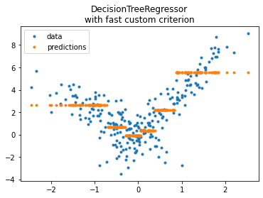
from mlinsights.mlmodel.piecewise_tree_regression_criterion_fast import SimpleRegressorCriterionFast
model3 = DecisionTreeRegressor(min_samples_leaf=100,
                              criterion=SimpleRegressorCriterionFast(X_train))
model3.fit(X_train, y_train)
pred = model3.predict(X_test)
pred[:5]

array([ 2.65757699,  0.37665413, -0.07967816,  0.37665413,  5.57229226])

fig, ax = plt.subplots(1, 1)
ax.plot(X_test[:, 0], y_test, ".", label='data')
ax.plot(X_test[:, 0], pred, ".", label="predictions")
ax.set_title("DecisionTreeRegressor\nwith fast custom criterion")
ax.legend();

%timeit model3.fit(X_train, y_train)

676 µs ± 48.8 µs per loop (mean ± std. dev. of 7 runs, 1000 loops each)

Much better even though this implementation is currently 3, 4 times slower than scikit-learn’s. Let’s check with a datasets three times bigger to see if it is a fix cost or a cost.

import numpy
X_train3 = numpy.vstack([X_train, X_train, X_train])
y_train3 = numpy.hstack([y_train, y_train, y_train])

X_train.shape, X_train3.shape, y_train3.shape

((750, 1), (2250, 1), (2250,))

%timeit model.fit(X_train3, y_train3)

1.36 ms ± 57 µs per loop (mean ± std. dev. of 7 runs, 1000 loops each)

The criterion needs to be reinstanciated since it depends on the features X. The computation does not but the design does. This was introduced to compare the current output with a decision tree optimizing for a piecewise linear regression and not a stepwise regression.

try:
    model3.fit(X_train3, y_train3)
except Exception as e:
    print(e)

X.shape=[750, 1, 0, 0, 0, 0, 0, 0] -- y.shape=[2250, 1, 0, 0, 0, 0, 0, 0]

model3 = DecisionTreeRegressor(min_samples_leaf=100,
                              criterion=SimpleRegressorCriterionFast(X_train3))
%timeit model3.fit(X_train3, y_train3)

2.03 ms ± 159 µs per loop (mean ± std. dev. of 7 runs, 100 loops each)

Still almost 2 times slower but of the same order of magnitude. We could go further and investigate why or continue and introduce a criterion which optimizes a piecewise linear regression instead of a stepwise regression.

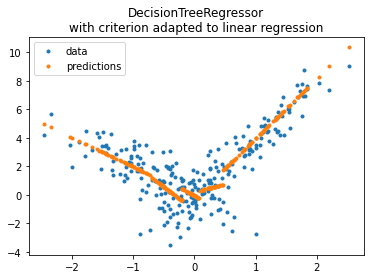
Criterion adapted for a linear regression

The previous examples are all about decision trees which approximates a function by a stepwise function. On every interval , the model optimizes and finds the best constant (= the average) approxmating the function on this interval. We would to like to approximate the function by a regression line and not a constant anymore. It means minimizing . Doing this require to change the criterion used to split the space of feature into buckets and the prediction function of the decision tree which now needs to return a dot product.

from mlinsights.mlmodel.piecewise_tree_regression import PiecewiseTreeRegressor
piece = PiecewiseTreeRegressor(criterion='mselin', min_samples_leaf=100)
piece.fit(X_train, y_train)

PiecewiseTreeRegressor(min_samples_leaf=100)

pred = piece.predict(X_test)
pred[:5]

array([3.80559618, 0.45086204, 0.42563158, 0.44940565, 3.57423704])

fig, ax = plt.subplots(1, 1)
ax.plot(X_test[:, 0], y_test, ".", label='data')
ax.plot(X_test[:, 0], pred, ".", label="predictions")
ax.set_title("DecisionTreeRegressor\nwith criterion adapted to linear regression")
ax.legend();

The coefficients for the linear regressions are kept into the following attribute:

piece.betas_

array([[-2.05163528, -0.07590713],
       [-3.28097357, -1.07747849],
       [-2.37373495, -0.05126022],
       [ 1.10248486,  0.20358196],
       [ 4.21766561, -0.2568136 ]])

Mapped to the following leaves:

piece.leaves_index_, piece.leaves_mapping_

([1, 4, 5, 7, 8], {1: 745, 4: 746, 3: 748, 0: 749, 2: 739})

We can get the leave each observation falls into:

piece.predict_leaves(X_test)[:5]

array([0, 3, 2, 3, 4])

The training is quite slow as it is training many linear regression each time a split is evaluated.

%timeit piece.fit(X_train, y_train)

26.9 ms ± 1.98 ms per loop (mean ± std. dev. of 7 runs, 10 loops each)

%timeit piece.fit(X_train3, y_train3)

105 ms ± 5.26 ms per loop (mean ± std. dev. of 7 runs, 10 loops each)

It works but it is slow, slower than the slow implementation of the standard criterion for decision tree regression.

Next

PR Model trees (M5P and co) and issue Model trees (M5P) propose an implementation a piecewise regression with any kind of regression model. It is based on Building Model Trees. It fits many models to find the best splits and should be slower than this implementation in the case of a decision tree regressor associated with linear regressions.