Regression with confidence interval#

Links: notebook, html, PDF, python, slides, GitHub

The notebook computes confidence intervals with bootstrapping and quantile regression on a simple problem.

from jyquickhelper import add_notebook_menu
add_notebook_menu()

%matplotlib inline

import warnings
warnings.simplefilter("ignore")

Some data #

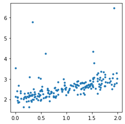
The data follows the formula: $y = \frac{X}{2} + 2 + \epsilon_1 + \eta \epsilon_2$ . Noises follows the laws $\epsilon_1 \sim \mathcal{N}(0, 0.2)$ , $\epsilon_2 \sim \mathcal{N}(1, 1)$ , $\eta \sim \mathcal{B}(2, 0.0.5)$ . The second part of the noise adds some bigger noise but not always.

from numpy.random import randn, binomial, rand
N = 200
X = rand(N, 1) * 2
eps = randn(N, 1) * 0.2
eps2 = randn(N, 1) + 1
bin = binomial(2, 0.05, size=(N, 1))
y = (0.5 * X + eps + 2 + eps2 * bin).ravel()

import matplotlib.pyplot as plt
fig, ax = plt.subplots(1, 1, figsize=(4, 4))
ax.plot(X, y, '.');

../_images/regression_confidence_interval_6_0.png

from sklearn.model_selection import train_test_split
X_train, X_test, y_train, y_test = train_test_split(X, y)

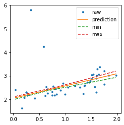
Confidence interval with a linear regression #

The object fits many times the same learner, every training is done on a resampling of the training dataset.

from mlinsights.mlmodel import IntervalRegressor
from sklearn.linear_model import LinearRegression

lin = IntervalRegressor(LinearRegression())
lin.fit(X_train, y_train)

IntervalRegressor(estimator=LinearRegression())

import numpy
sorted_X = numpy.array(list(sorted(X_test)))
pred = lin.predict(sorted_X)
bootstrapped_pred = lin.predict_sorted(sorted_X)
min_pred = bootstrapped_pred[:, 0]
max_pred = bootstrapped_pred[:, bootstrapped_pred.shape[1]-1]

fig, ax = plt.subplots(1, 1, figsize=(4, 4))
ax.plot(X_test, y_test, '.', label="raw")
ax.plot(sorted_X, pred, label="prediction")
ax.plot(sorted_X, min_pred, '--', label="min")
ax.plot(sorted_X, max_pred, '--', label="max")
ax.legend();

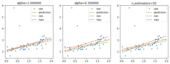
../_images/regression_confidence_interval_11_0.png

Higher confidence interval #

It is possible to use smaller resample of the training dataset or we can increase the number of resamplings.

lin2 = IntervalRegressor(LinearRegression(), alpha=0.3)
lin2.fit(X_train, y_train)

IntervalRegressor(alpha=0.3, estimator=LinearRegression())

lin3 = IntervalRegressor(LinearRegression(), n_estimators=50)
lin3.fit(X_train, y_train)

IntervalRegressor(estimator=LinearRegression(), n_estimators=50)

pred2 = lin2.predict(sorted_X)
bootstrapped_pred2 = lin2.predict_sorted(sorted_X)
min_pred2 = bootstrapped_pred2[:, 0]
max_pred2 = bootstrapped_pred2[:, bootstrapped_pred2.shape[1]-1]

pred3 = lin3.predict(sorted_X)
bootstrapped_pred3 = lin3.predict_sorted(sorted_X)
min_pred3 = bootstrapped_pred3[:, 0]
max_pred3 = bootstrapped_pred3[:, bootstrapped_pred3.shape[1]-1]

fig, ax = plt.subplots(1, 3, figsize=(12, 4))
ax[0].plot(X_test, y_test, '.', label="raw")
ax[0].plot(sorted_X, pred, label="prediction")
ax[0].plot(sorted_X, min_pred, '--', label="min")
ax[0].plot(sorted_X, max_pred, '--', label="max")
ax[0].legend()
ax[0].set_title("alpha=%f" % lin.alpha)
ax[1].plot(X_test, y_test, '.', label="raw")
ax[1].plot(sorted_X, pred2, label="prediction")
ax[1].plot(sorted_X, min_pred2, '--', label="min")
ax[1].plot(sorted_X, max_pred2, '--', label="max")
ax[1].set_title("alpha=%f" % lin2.alpha)
ax[1].legend()
ax[2].plot(X_test, y_test, '.', label="raw")
ax[2].plot(sorted_X, pred3, label="prediction")
ax[2].plot(sorted_X, min_pred3, '--', label="min")
ax[2].plot(sorted_X, max_pred3, '--', label="max")
ax[2].set_title("n_estimators=%d" % lin3.n_estimators)
ax[2].legend();

../_images/regression_confidence_interval_17_0.png

With decision trees #

from sklearn.tree import DecisionTreeRegressor
tree = IntervalRegressor(DecisionTreeRegressor(min_samples_leaf=10))
tree.fit(X_train, y_train)

IntervalRegressor(estimator=DecisionTreeRegressor(min_samples_leaf=10))

pred_tree = tree.predict(sorted_X)
b_pred_tree = tree.predict_sorted(sorted_X)
min_pred_tree = b_pred_tree[:, 0]
max_pred_tree = b_pred_tree[:, b_pred_tree.shape[1]-1]

fig, ax = plt.subplots(1, 1, figsize=(4, 4))
ax.plot(X_test, y_test, '.', label="raw")
ax.plot(sorted_X, pred_tree, label="prediction")
ax.plot(sorted_X, min_pred_tree, '--', label="min")
ax.plot(sorted_X, max_pred_tree, '--', label="max")
ax.set_title("Interval with trees")
ax.legend();

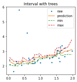
../_images/regression_confidence_interval_21_0.png

In that case, the prediction is very similar to the one a random forest would produce as it is an average of the predictions made by 10 trees.

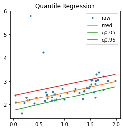
Regression quantile #

The last way tries to fit two regressions for quantiles 0.05 and 0.95.

from mlinsights.mlmodel import QuantileLinearRegression
m = QuantileLinearRegression()
q1 = QuantileLinearRegression(quantile=0.05)
q2 = QuantileLinearRegression(quantile=0.95)
for model in [m, q1, q2]:
    model.fit(X_train, y_train)

fig, ax = plt.subplots(1, 1, figsize=(4, 4))
ax.plot(X_test, y_test, '.', label="raw")

for label, model in [('med', m), ('q0.05', q1), ('q0.95', q2)]:
    p = model.predict(sorted_X)
    ax.plot(sorted_X, p, label=label)
ax.set_title("Quantile Regression")
ax.legend();

../_images/regression_confidence_interval_25_0.png

With a non linear model… but the model QuantileMLPRegressor only implements the regression with quantile 0.5.

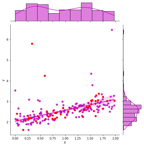
With seaborn #

It uses a theoritical way to compute the confidence interval by computing the confidence interval on the parameters first.

import seaborn as sns
import pandas

df_train = pandas.DataFrame(dict(X=X_train.ravel(), y=y_train))
g = sns.jointplot("X", "y", data=df_train, kind="reg", color="m", height=7)
g.ax_joint.plot(X_test, y_test, 'ro');

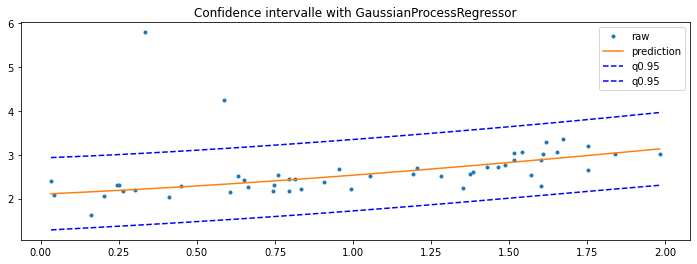
../_images/regression_confidence_interval_28_0.png

GaussianProcessRegressor #

Last option with this example Gaussian Processes regression: basic introductory example which computes the standard deviation for every prediction. It can then be used to show an interval confidence.

from sklearn.gaussian_process import GaussianProcessRegressor
from sklearn.gaussian_process.kernels import RBF, ConstantKernel as C, DotProduct, WhiteKernel

kernel = C(1.0, (1e-3, 1e3)) * RBF(10, (1e-2, 1e2)) + WhiteKernel()
gp = GaussianProcessRegressor(kernel=kernel, n_restarts_optimizer=9)
gp.fit(X_train, y_train)

GaussianProcessRegressor(kernel=1**2 * RBF(length_scale=10) + WhiteKernel(noise_level=1),
                         n_restarts_optimizer=9)

y_pred, sigma = gp.predict(sorted_X, return_std=True)

fig, ax = plt.subplots(1, 1, figsize=(12, 4))
ax.plot(X_test, y_test, '.', label="raw")
ax.plot(sorted_X, y_pred, label="prediction")
ax.plot(sorted_X, y_pred + sigma * 1.96, 'b--', label="q0.95")
ax.plot(sorted_X, y_pred - sigma * 1.96, 'b--', label="q0.95")
ax.set_title("Confidence intervalle with GaussianProcessRegressor")
ax.legend();

../_images/regression_confidence_interval_32_0.png

Regression with confidence interval#

Some data#

Confidence interval with a linear regression#

Higher confidence interval#

With decision trees#

Regression quantile#

With seaborn#

GaussianProcessRegressor#