Note
Click here to download the full example code
Benchmark Random Forests, Tree Ensemble, (AoS and SoA)#
The script compares different implementations for the operator TreeEnsembleRegressor.
baseline: RandomForestRegressor from scikit-learn
ort: onnxruntime,
mlprodict: an implementation based on an array of structures, every structure describes a node,
mlprodict2 similar implementation but instead of having an array of structures, it relies on a structure of arrays, it parallelizes by blocks of 128 observations and inside every block, goes through trees then through observations (double loop),
mlprodict3: parallelizes by trees, this implementation is faster when the depth is higher than 10.
A structure of arrays has better performance: Case study: Comparing Arrays of Structures and Structures of Arrays Data Layouts for a Compute-Intensive Loop. See also AoS and SoA.
Profile the execution
py-spy can be used to profile the execution of a program. The profile is more informative if the code is compiled with debug information.
py-spy record --native -r 10 -o plot_random_forest_reg.svg -- python plot_random_forest_reg.py
Import#
import warnings
from time import perf_counter as time
from multiprocessing import cpu_count
import numpy
from numpy.random import rand
from numpy.testing import assert_almost_equal
import pandas
import matplotlib.pyplot as plt
from sklearn import config_context
from sklearn.ensemble import RandomForestRegressor
from sklearn.utils._testing import ignore_warnings
from skl2onnx import convert_sklearn
from skl2onnx.common.data_types import FloatTensorType
from onnxruntime import InferenceSession
from mlprodict.onnxrt import OnnxInference
Available optimisation on this machine.
from mlprodict.testing.experimental_c_impl.experimental_c import code_optimisation
print(code_optimisation())
AVX-omp=8
Versions#
def version():
    from datetime import datetime
    import sklearn
    import numpy
    import onnx
    import onnxruntime
    import skl2onnx
    import mlprodict
    df = pandas.DataFrame([
        {"name": "date", "version": str(datetime.now())},
        {"name": "numpy", "version": numpy.__version__},
        {"name": "scikit-learn", "version": sklearn.__version__},
        {"name": "onnx", "version": onnx.__version__},
        {"name": "onnxruntime", "version": onnxruntime.__version__},
        {"name": "skl2onnx", "version": skl2onnx.__version__},
        {"name": "mlprodict", "version": mlprodict.__version__},
    ])
    return df


version()
Implementations to benchmark#
def fcts_model(X, y, max_depth, n_estimators, n_jobs):
    "RandomForestClassifier."
    rf = RandomForestRegressor(max_depth=max_depth, n_estimators=n_estimators,
                               n_jobs=n_jobs)
    rf.fit(X, y)

    initial_types = [('X', FloatTensorType([None, X.shape[1]]))]
    onx = convert_sklearn(rf, initial_types=initial_types)
    sess = InferenceSession(onx.SerializeToString())
    outputs = [o.name for o in sess.get_outputs()]
    oinf = OnnxInference(onx, runtime="python")
    oinf.sequence_[0].ops_._init(numpy.float32, 1)
    name = outputs[0]
    oinf2 = OnnxInference(onx, runtime="python")
    oinf2.sequence_[0].ops_._init(numpy.float32, 2)
    oinf3 = OnnxInference(onx, runtime="python")
    oinf3.sequence_[0].ops_._init(numpy.float32, 3)

    def predict_skl_predict(X, model=rf):
        return rf.predict(X)

    def predict_onnxrt_predict(X, sess=sess):
        return sess.run(outputs[:1], {'X': X})[0]

    def predict_onnx_inference(X, oinf=oinf):
        return oinf.run({'X': X})[name]

    def predict_onnx_inference2(X, oinf2=oinf2):
        return oinf2.run({'X': X})[name]

    def predict_onnx_inference3(X, oinf3=oinf3):
        return oinf3.run({'X': X})[name]

    return {'predict': (
        predict_skl_predict, predict_onnxrt_predict,
        predict_onnx_inference, predict_onnx_inference2,
        predict_onnx_inference3)}
Benchmarks#
def allow_configuration(**kwargs):
    return True


def bench(n_obs, n_features, max_depths, n_estimatorss, n_jobss,
          methods, repeat=10, verbose=False):
    res = []
    for nfeat in n_features:

        ntrain = 50000
        X_train = numpy.empty((ntrain, nfeat)).astype(numpy.float32)
        X_train[:, :] = rand(ntrain, nfeat)[:, :]
        eps = rand(ntrain) - 0.5
        y_train = X_train.sum(axis=1) + eps

        for n_jobs in n_jobss:
            for max_depth in max_depths:
                for n_estimators in n_estimatorss:
                    fcts = fcts_model(X_train, y_train,
                                      max_depth, n_estimators, n_jobs)

                    for n in n_obs:
                        for method in methods:

                            fct1, fct2, fct3, fct4, fct5 = fcts[method]

                            if not allow_configuration(
                                    n=n, nfeat=nfeat, max_depth=max_depth,
                                    n_estimator=n_estimators, n_jobs=n_jobs,
                                    method=method):
                                continue

                            obs = dict(n_obs=n, nfeat=nfeat,
                                       max_depth=max_depth,
                                       n_estimators=n_estimators,
                                       method=method,
                                       n_jobs=n_jobs)

                            # creates different inputs to avoid caching
                            Xs = []
                            for r in range(repeat):
                                x = numpy.empty((n, nfeat))
                                x[:, :] = rand(n, nfeat)[:, :]
                                Xs.append(x.astype(numpy.float32))

                            # measures the baseline
                            with config_context(assume_finite=True):
                                st = time()
                                repeated = 0
                                for X in Xs:
                                    p1 = fct1(X)
                                    repeated += 1
                                    if time() - st >= 1:
                                        break  # stops if longer than a second
                                end = time()
                                obs["time_skl"] = (end - st) / repeated

                            # measures the new implementation
                            st = time()
                            r2 = 0
                            for X in Xs:
                                p2 = fct2(X)
                                r2 += 1
                                if r2 >= repeated:
                                    break
                            end = time()
                            obs["time_ort"] = (end - st) / r2

                            # measures the other new implementation
                            st = time()
                            r2 = 0
                            for X in Xs:
                                p2 = fct3(X)
                                r2 += 1
                                if r2 >= repeated:
                                    break
                            end = time()
                            obs["time_mlprodict"] = (end - st) / r2

                            # measures the other new implementation 2
                            st = time()
                            r2 = 0
                            for X in Xs:
                                p2 = fct4(X)
                                r2 += 1
                                if r2 >= repeated:
                                    break
                            end = time()
                            obs["time_mlprodict2"] = (end - st) / r2

                            # measures the other new implementation 3
                            st = time()
                            r2 = 0
                            for X in Xs:
                                p2 = fct5(X)
                                r2 += 1
                                if r2 >= repeated:
                                    break
                            end = time()
                            obs["time_mlprodict3"] = (end - st) / r2

                            # final
                            res.append(obs)
                            if verbose and (len(res) % 1 == 0 or n >= 10000):
                                print("bench", len(res), ":", obs)

                            # checks that both produce the same outputs
                            if n <= 10000:
                                if len(p1.shape) == 1 and len(p2.shape) == 2:
                                    p2 = p2.ravel()
                                try:
                                    assert_almost_equal(
                                        p1.ravel(), p2.ravel(), decimal=5)
                                except AssertionError as e:
                                    warnings.warn(str(e))
    return res
Graphs#
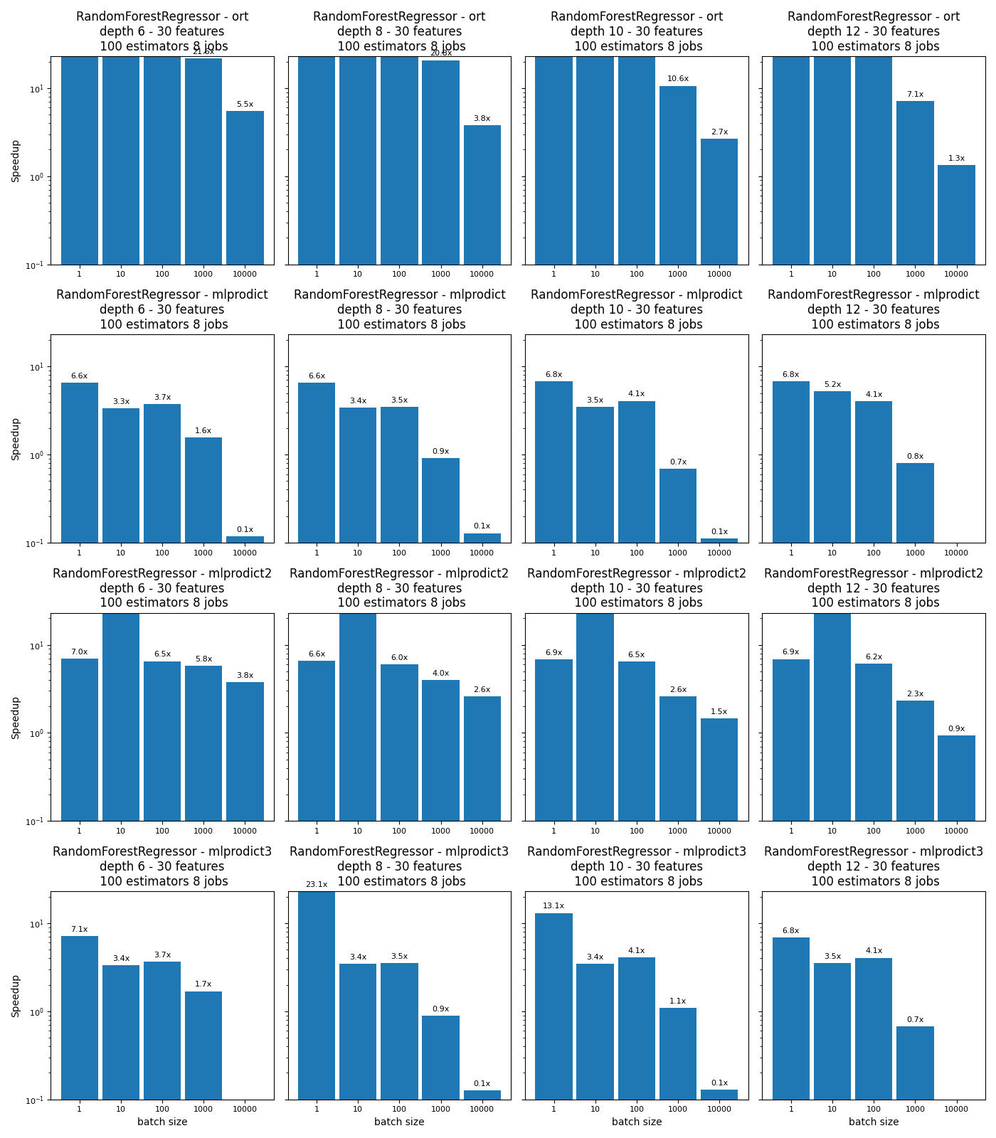
def plot_rf_models(dfr):

    def autolabel(ax, rects):
        for rect in rects:
            height = rect.get_height()
            ax.annotate(f'{height:1.1f}x',
                        xy=(rect.get_x() + rect.get_width() / 2, height),
                        xytext=(0, 3),  # 3 points vertical offset
                        textcoords="offset points",
                        ha='center', va='bottom',
                        fontsize=8)

    engines = [_.split('_')[-1] for _ in dfr.columns if _.startswith("time_")]
    engines = [_ for _ in engines if _ != 'skl']
    for engine in engines:
        dfr[f"speedup_{engine}"] = dfr["time_skl"] / dfr[f"time_{engine}"]
    print(dfr.tail().T)

    ncols = 4
    fig, axs = plt.subplots(len(engines), ncols, figsize=(
        14, 4 * len(engines)), sharey=True)

    row = 0
    for row, engine in enumerate(engines):
        pos = 0
        name = f"RandomForestRegressor - {engine}"
        for max_depth in sorted(set(dfr.max_depth)):
            for nf in sorted(set(dfr.nfeat)):
                for est in sorted(set(dfr.n_estimators)):
                    for n_jobs in sorted(set(dfr.n_jobs)):
                        sub = dfr[(dfr.max_depth == max_depth) &
                                  (dfr.nfeat == nf) &
                                  (dfr.n_estimators == est) &
                                  (dfr.n_jobs == n_jobs)]
                        ax = axs[row, pos]
                        labels = sub.n_obs
                        means = sub[f"speedup_{engine}"]

                        x = numpy.arange(len(labels))
                        width = 0.90

                        rects1 = ax.bar(x, means, width, label='Speedup')
                        if pos == 0:
                            ax.set_yscale('log')
                            ax.set_ylim([0.1, max(dfr[f"speedup_{engine}"])])

                        if pos == 0:
                            ax.set_ylabel('Speedup')
                        ax.set_title(
                            '%s\ndepth %d - %d features\n %d estimators %d '
                            'jobs' % (name, max_depth, nf, est, n_jobs))
                        if row == len(engines) - 1:
                            ax.set_xlabel('batch size')
                        ax.set_xticks(x)
                        ax.set_xticklabels(labels)
                        autolabel(ax, rects1)
                        for tick in ax.xaxis.get_major_ticks():
                            tick.label.set_fontsize(8)
                        for tick in ax.yaxis.get_major_ticks():
                            tick.label.set_fontsize(8)
                        pos += 1

    fig.tight_layout()
    return fig, ax
Run benchs#
@ignore_warnings(category=FutureWarning)
def run_bench(repeat=100, verbose=False):
    n_obs = [1, 10, 100, 1000, 10000]
    methods = ['predict']
    n_features = [30]
    max_depths = [6, 8, 10, 12]
    n_estimatorss = [100]
    n_jobss = [cpu_count()]

    start = time()
    results = bench(n_obs, n_features, max_depths, n_estimatorss, n_jobss,
                    methods, repeat=repeat, verbose=verbose)
    end = time()

    results_df = pandas.DataFrame(results)
    print("Total time = %0.3f sec cpu=%d\n" % (end - start, cpu_count()))

    # plot the results
    return results_df


name = "plot_random_forest_reg"
df = run_bench(verbose=True)
df.to_csv(f"{name}.csv", index=False)
df.to_excel(f"{name}.xlsx", index=False)
fig, ax = plot_rf_models(df)
fig.savefig(f"{name}.png")
plt.show()
bench 1 : {'n_obs': 1, 'nfeat': 30, 'max_depth': 6, 'n_estimators': 100, 'method': 'predict', 'n_jobs': 8, 'time_skl': 0.04274427462466216, 'time_ort': 6.223437473333131e-05, 'time_mlprodict': 0.006505213750642724, 'time_mlprodict2': 0.006133636333591615, 'time_mlprodict3': 0.006030462420312688}
bench 2 : {'n_obs': 10, 'nfeat': 30, 'max_depth': 6, 'n_estimators': 100, 'method': 'predict', 'n_jobs': 8, 'time_skl': 0.04139167800080031, 'time_ort': 0.0003842888819053769, 'time_mlprodict': 0.012418290758505464, 'time_mlprodict2': 0.0001894340803846717, 'time_mlprodict3': 0.012340408395975827}
bench 3 : {'n_obs': 100, 'nfeat': 30, 'max_depth': 6, 'n_estimators': 100, 'method': 'predict', 'n_jobs': 8, 'time_skl': 0.045885168090039355, 'time_ort': 0.00047946963670917535, 'time_mlprodict': 0.012305136224974624, 'time_mlprodict2': 0.007038850136185912, 'time_mlprodict3': 0.012557338637469167}
bench 4 : {'n_obs': 1000, 'nfeat': 30, 'max_depth': 6, 'n_estimators': 100, 'method': 'predict', 'n_jobs': 8, 'time_skl': 0.06382088743703207, 'time_ort': 0.0029533385022659786, 'time_mlprodict': 0.041088564685196616, 'time_mlprodict2': 0.011018224620784167, 'time_mlprodict3': 0.03776891368761426}
bench 5 : {'n_obs': 10000, 'nfeat': 30, 'max_depth': 6, 'n_estimators': 100, 'method': 'predict', 'n_jobs': 8, 'time_skl': 0.08683001716660026, 'time_ort': 0.015782713249791414, 'time_mlprodict': 0.736361120827496, 'time_mlprodict2': 0.02297877207941686, 'time_mlprodict3': 0.9753920404182281}
bench 6 : {'n_obs': 1, 'nfeat': 30, 'max_depth': 8, 'n_estimators': 100, 'method': 'predict', 'n_jobs': 8, 'time_skl': 0.04192163804448986, 'time_ort': 6.702054330768685e-05, 'time_mlprodict': 0.006381189208089684, 'time_mlprodict2': 0.006371027251589112, 'time_mlprodict3': 0.0018173234566347674}
bench 7 : {'n_obs': 10, 'nfeat': 30, 'max_depth': 8, 'n_estimators': 100, 'method': 'predict', 'n_jobs': 8, 'time_skl': 0.042143816623138264, 'time_ort': 0.0006803655414842069, 'time_mlprodict': 0.012322351249167696, 'time_mlprodict2': 0.000588648957394374, 'time_mlprodict3': 0.012241991668512734}
bench 8 : {'n_obs': 100, 'nfeat': 30, 'max_depth': 8, 'n_estimators': 100, 'method': 'predict', 'n_jobs': 8, 'time_skl': 0.04502972130380247, 'time_ort': 0.0008717101705058113, 'time_mlprodict': 0.012853026612783256, 'time_mlprodict2': 0.007448452828532975, 'time_mlprodict3': 0.012698329914280253}
bench 9 : {'n_obs': 1000, 'nfeat': 30, 'max_depth': 8, 'n_estimators': 100, 'method': 'predict', 'n_jobs': 8, 'time_skl': 0.0660240198703832, 'time_ort': 0.003177096186846029, 'time_mlprodict': 0.07283168956200825, 'time_mlprodict2': 0.016596586247032974, 'time_mlprodict3': 0.07363988437282387}
bench 10 : {'n_obs': 10000, 'nfeat': 30, 'max_depth': 8, 'n_estimators': 100, 'method': 'predict', 'n_jobs': 8, 'time_skl': 0.0887689823381758, 'time_ort': 0.02344617566753489, 'time_mlprodict': 0.6914812588268736, 'time_mlprodict2': 0.033903778491852186, 'time_mlprodict3': 0.7002630396649087}
bench 11 : {'n_obs': 1, 'nfeat': 30, 'max_depth': 10, 'n_estimators': 100, 'method': 'predict', 'n_jobs': 8, 'time_skl': 0.04237027762671156, 'time_ort': 0.00010302728818108638, 'time_mlprodict': 0.00621231846162118, 'time_mlprodict2': 0.006183585418815103, 'time_mlprodict3': 0.0032372772499608495}
bench 12 : {'n_obs': 10, 'nfeat': 30, 'max_depth': 10, 'n_estimators': 100, 'method': 'predict', 'n_jobs': 8, 'time_skl': 0.043248251958478555, 'time_ort': 0.0009172522938267017, 'time_mlprodict': 0.012395918873759607, 'time_mlprodict2': 0.000969078416043582, 'time_mlprodict3': 0.01256808833568357}
bench 13 : {'n_obs': 100, 'nfeat': 30, 'max_depth': 10, 'n_estimators': 100, 'method': 'predict', 'n_jobs': 8, 'time_skl': 0.05404166847246846, 'time_ort': 0.001302548261408351, 'time_mlprodict': 0.013250650004728845, 'time_mlprodict2': 0.008324564207884433, 'time_mlprodict3': 0.013145678002681387}
bench 14 : {'n_obs': 1000, 'nfeat': 30, 'max_depth': 10, 'n_estimators': 100, 'method': 'predict', 'n_jobs': 8, 'time_skl': 0.06621509043907281, 'time_ort': 0.006222726879059337, 'time_mlprodict': 0.09657030319067417, 'time_mlprodict2': 0.02533866231533466, 'time_mlprodict3': 0.06031203343445668}
bench 15 : {'n_obs': 10000, 'nfeat': 30, 'max_depth': 10, 'n_estimators': 100, 'method': 'predict', 'n_jobs': 8, 'time_skl': 0.09021130333227727, 'time_ort': 0.03384415574449425, 'time_mlprodict': 0.8070350550891211, 'time_mlprodict2': 0.0613647821592167, 'time_mlprodict3': 0.7027815164183266}
bench 16 : {'n_obs': 1, 'nfeat': 30, 'max_depth': 12, 'n_estimators': 100, 'method': 'predict', 'n_jobs': 8, 'time_skl': 0.04291177958172435, 'time_ort': 8.826204187547167e-05, 'time_mlprodict': 0.006334640498001439, 'time_mlprodict2': 0.006213610497070476, 'time_mlprodict3': 0.006276590705965646}
bench 17 : {'n_obs': 10, 'nfeat': 30, 'max_depth': 12, 'n_estimators': 100, 'method': 'predict', 'n_jobs': 8, 'time_skl': 0.043733895477919796, 'time_ort': 0.0010634556048266265, 'time_mlprodict': 0.008363155212820224, 'time_mlprodict2': 0.0012041385255187101, 'time_mlprodict3': 0.012366141997399214}
bench 18 : {'n_obs': 100, 'nfeat': 30, 'max_depth': 12, 'n_estimators': 100, 'method': 'predict', 'n_jobs': 8, 'time_skl': 0.05578579688962135, 'time_ort': 0.0017745679425489572, 'time_mlprodict': 0.013762781221885234, 'time_mlprodict2': 0.009069721499044035, 'time_mlprodict3': 0.013756523555558588}
bench 19 : {'n_obs': 1000, 'nfeat': 30, 'max_depth': 12, 'n_estimators': 100, 'method': 'predict', 'n_jobs': 8, 'time_skl': 0.06995020406320691, 'time_ort': 0.009843397132741908, 'time_mlprodict': 0.08748375320186218, 'time_mlprodict2': 0.030305100868766508, 'time_mlprodict3': 0.10346798666287213}
bench 20 : {'n_obs': 10000, 'nfeat': 30, 'max_depth': 12, 'n_estimators': 100, 'method': 'predict', 'n_jobs': 8, 'time_skl': 0.09470866154879332, 'time_ort': 0.07119774518915536, 'time_mlprodict': 1.0159253080968151, 'time_mlprodict2': 0.10117462536701086, 'time_mlprodict3': 1.08055495608344}
Total time = 389.856 sec cpu=8

                            15         16        17        18        19
n_obs                        1         10       100      1000     10000
nfeat                       30         30        30        30        30
max_depth                   12         12        12        12        12
n_estimators               100        100       100       100       100
method                 predict    predict   predict   predict   predict
n_jobs                       8          8         8         8         8
time_skl              0.042912   0.043734  0.055786   0.06995  0.094709
time_ort              0.000088   0.001063  0.001775  0.009843  0.071198
time_mlprodict        0.006335   0.008363  0.013763  0.087484  1.015925
time_mlprodict2       0.006214   0.001204   0.00907  0.030305  0.101175
time_mlprodict3       0.006277   0.012366  0.013757  0.103468  1.080555
speedup_ort         486.186119  41.124326  31.43627  7.106307   1.33022
speedup_mlprodict     6.774146   5.229354  4.053381  0.799579  0.093224
speedup_mlprodict2    6.906094  36.319655  6.150773  2.308199  0.936091
speedup_mlprodict3    6.836797   3.536584  4.055225  0.676056  0.087648
somewhere/workspace/mlprodict/mlprodict_UT_39_std/_doc/examples/plot_opml_random_forest_reg.py:323: MatplotlibDeprecationWarning: The label function was deprecated in Matplotlib 3.1 and will be removed in 3.8. Use Tick.label1 instead.
  tick.label.set_fontsize(8)
somewhere/workspace/mlprodict/mlprodict_UT_39_std/_doc/examples/plot_opml_random_forest_reg.py:325: MatplotlibDeprecationWarning: The label function was deprecated in Matplotlib 3.1 and will be removed in 3.8. Use Tick.label1 instead.
  tick.label.set_fontsize(8)
Total running time of the script: ( 6 minutes 41.805 seconds)